Introduction

The cache, capture real dynamic behaviour of the Internet. That is what makes it hard to understand. Until researchers understand the dynamics and behaviour of the Internet, caching will also not be understood, some material is here. However, not all is lost. The working premise of work such as this is; if one can store the data closer to the consumers, time to consume the data can be lowered. This is because the data is closer in distance (actual km) and hence the network round trip times will be lower. Also loads on the network and servers between the cache and server can be reduced, assuming the cache has some efficacy. There will be some savings in peering costs too, as lower amounts of data are transferred. The cost is the storage infrastructure, energy and maintenance costs. If a third party is used, of which there are many today, payments need to be made. Such operators are referred to as content distributors where larger scale storage is provided over a country or continent.

The introduction of caching has to be done carefully, not only in terms of location, but also size, a too small cache will add delays, only for the requested items not to be found, a cache “miss”. However the cost of redirecting, intercepting the original request to a server, searching in the cost, managing it will add to the latency, therefore introducing a poorly dimensioned, or sized cache could worsen performance. Performance particularly in terms of latency, point (iii) above. On the other hand, a too large cache may be costly, in terms of equipment, which is much more than the sales cost in running systems. Also larger systems are more prone to failure and require regular maintenance, as well as needing more power. Therefore it is important to select the correct placement and sizing for the network cache [Bjurling14, Marsh14].

Background

Now we will spend some paragraphs explaining the problem domain. In terms, the first assumption is that intercepting the request, locating the item in the cache and serving it back to the user requires less time than the traditional client-server connection. However, if locating items in a cache requires more time, then caching will not be effective as a time reduction mechanism. This is often not an straightforward decision (or indeed calculation) to make as the number of dependencies is large. One has to calculate the relative win/loss in the cached and non-cached path, including the link speeds between the client, server and caches, also one has to consider the size of the item as well as the access speed to the caches. Also it has to be shown that a cache by cache search requires less time than a straightforward end-to-end request. Although this could be done in the static case, a further non-static factor is the relative congestion on the intervening links in the cached and non-cached systems should be included in the calculation. Also potential contention to shared resources tends not to be a deterministic quantity. This is complex before we even consider a single long round trip time TCP connection versus several shorter round trip time connections.

With the increase of global network traffic, particularly video, network caching has been thus far well utilised within CDNs for download streaming. From an energy efficiency perspective, it is not clear, whether this is the best option, is it better to store items closer to the user, or within a data center and redistribute. That is because data centers are very energy efficient, but has the cost of the transferring the bits across a network (assuming the data center is somewhat remote). Data in a CDN or local-ish cache, might be less efficient per bit, but is closer to the user, incurring less transmission costs.

Goals of caching

Content caching is highly beneficial from the perspective of both network operators and end users. If one can store content closer to its consumers, the time to access and retrieve the content is lowered, since it is closer in distance (actual km) and network hops leading to lower round trip times. Additionally, loads on the network between the cache and server are reduced, assuming the cache has non-zero efficacy. In particular, caching mechanisms can reduce i) the load on servers by replicating popular content to caches in multiple locations, ii) the load on heavy utilized links, as many flows aggregate towards popular servers, and iii) the latency for end users, as the content is closer in network terms. Furthermore, there will be savings in peering costs, as lower amounts of data are transferred across domains. The downsides are the cost for storage infrastructure, energy, and maintenance — usually already catered for in most Content Delivery Networks (CDNs) — and the extra complexity introduced into the network infrastructure to manage the caches.

1. Delay reduction
2. Load reduction
3. Peering cost reduction
4. Localised content

There are whole other dimensions to the problem as well. One is the time dependent popularity of the items. Popularity not only increases or decreases over time but in VoD cases acyclic behavior exists. This is where one show prompts viewers to search for previous (or related) shows. The popularity dynamics are also influenced by social media, for example groups of people posting links to images or videos. Another dimension is space, where items are more or less popular dependent on the region. Language specific content is clearly an example of spatial diversity. The size of the objects has a major impact on the cache occupancy, is it better to store a 1×100 unit item or 100×1 unit items? The replacement policy of each cache is important too, should one replace the oldest, least frequency or random item? Although the least frequently used item may seem most appropriate, it is more computationally expensive to calculate than the others. In the cellular case (3 previously)above, the time dependent characteristics may also be a factor, not because the cache is after the wireless (often poorer) link, rather the size of the item becomes significant, larger items being more prone to time dependent impairments during wireless transmission. This impacts on the perceived Quality of Experience (QoE) for the user.

A cache captures complex dynamics

It is a very benign thing, basically contiguous memory, but a cache captures complex dynamics. That is the time varying populations and dynamics of the accessible files on the Internet and their requestors. Add the topology of the network, policies affecting the network path choice, overload mechanisms plus failures the cache captures many, but not all, of these dynamics. Parallels can be draw with web caching, which is still a complex dynamic, but of a single user. Another parallel can be drawn with buffering in the Internet, albeit on shorter time scales.

Content caching preliminaries

In general, two models of content distribution exist: one is a push-based model where popular items are pushed out into the infrastructure, which is used by providers who estimate which items will be frequently consumed in the near future. Examples include highly publicized or popular media such as operating system releases. Typically the content tends to be larger than a web page in the order of several hundreds of megabytes. The other model is pull-based, where the request dynamics influence the items within the caches. Pull-based systems eventually store the most accessed items or more recently accessed items over a given time period.

An important evaluation criterion is the response time of a cache, which is stochastic, typically bimodally distributed. One modality is the time to find an item in the cache, a hit. 

Dynamic content

Changes over time (popularity not constant) new items may not receive many searches and retrievals, since they are not known. Since the advent of social media, however, a small fraction the existing and new content may become very popular, so called ‘going viral’

Hardware factors

The retrieval speed of content depends on the speeds of the Internet connections, traffic on the links and the hardware itself. Clearly disk access speeds have changed with solid state devices, hybrids which are mechanical and SSD / NVRAMe disks now exist. HW speeds, data structure, SSD, disks, placement, difference in access times are important, particularly their relative access / storage ratios. Caching is the mitigation technique used in CPU L1/2 architecture.

Content push or pull

Two models of distribution exist. One is push-based where popular items are pushed out into the infrastructure, this model is used by providers who know items will be popular and consumed in the not too distant future. Examples include highly publicized media or operating system releases/updates. Typically the content tends to be larger, several hundreds of megabytes. This means that some of the content in the cache is predetermined by the entity pushing out the content, exclusively so in some cases. The other model is pull-based, where the dynamics of the requests decide on the items within the caches. Although more dynamic initially, pull-based systems eventually store the most accessed items over a given time period. An interesting research issue, is what is the optimal time for windowing in a caching system? In other words, over how long a time period should one try and predict the future behavior? Clearly the traffic patterns are well known through EPG guides and daily human swings, however on the microscopic scale it is nigh on impossible to make predictions, but is there a more realistic time scale to analyze the patterns and trends and make sensible network management decisions to cope with temporal trends, viral videos being such a topic.

Content size dependencies

Predicting which items to keep in a stored memory environment. items can be web retrieved objects such as html pages, mp3 files, video or software. The total size of the items will be larger than the total storage in the storage. Therefore some replacement algorithm will be needed.

The popularity of some of the items is known (or can be measured, estimated). Temporal dynamics exist. Spatial artifacts too, as different interests and languages will be evident, news in Greek will be more popular in Greece and Greek speaking populations. Network topology will be important too, but we can begin with a single storage. Object size is important, as many small items can be stored at the expense of smaller items. Timeliness is important too, as some media need to delivered “on-time”.

Delay measurements

Packets (flows, sessions) through a system encounter buffers and queues. Queues and buffers exist in systems to provide high capacity, by continually filling them whence the system has resources. Buffers also exist when the system is “busy” such as link being available or not. Although buffers can be good for high throughput data sessions, it can be to the detriment to time-sensitive sessions such as telephony, stock trading or machine control. Some sessions have rate control as well, such as the widely used transport protocol TCP, in the TCP/IP suite used in today’s Internet.

The idea is send a series of data through a network and form a distribution of delays. The distribution will represent different “paths” in the system, the data flows freely through the system, the data encounters some delays, or the data encounters several delays in series. We would like to be able to identify the sources of delays in the system, from analysis.

Measurement data as well as control systems and simulators are available to help us isolate some delays.

Techniques used in caching analysis

1. Sampling theory
2. Statistics. (PCA of best techniques)
3. Combinatorial analysis
4. Prediction
5. Estimation theory
6. Machine learning
7. Neural networks
8. Time series analysis
9. Visualisation (simulation)

A dynamic cache sizing example

Start with two arguments: QoE for user and cost for operator. Buffering events in media replay are commonplace and annoying. Where data is retrieved from a cache, an access miss will lead to longer round trip times as the server’s copy will be needed to replay the   video, and optionally copied into the cache.  Dynamics arise from the cache, as the requests of many clients at the cache, over differing link capacities, network locations, media types and time scales induce complex behaviors. In essence, the cache captures a snapshot of the users and the items available plus their dynamics.  Therefore in this work we show how to dimension and regulate a network cache, based on the request patterns from the clients.  A reduction in the variance in a cache hit rate means a reduction in the variance for an application.  Our contribution in this work is the regulation of a single cache’s hit rate through size changes using a standard controller.  We have evaluated our approach with real workloads taken from a 3G access network, and show that the reduction in the hit rate can be up to 30\% rather than the commonly used Zipf-like workloads. 

In this section we advocate enhancing data caching mechanisms by an adaptive control algorithm. Our contribution is twofold: We start by studying the popularity of MIME types in a rich real-world dataset from a nation-wide 3G access network and propose then a single cache control algorithm. We focus on the most popular MIME types, since the volumes taken by applications (updates, games) and video predominate the Internet traffic 

Moreover, the dominance of these data types is expected to further grow in the next couple of years, e.g., it has been predicted that video will amount to more than 60\% of the total volume of total Internet traffic, both on fixed networks and increasingly also on mobile networks [Cisco].

The organization of the rest of this paper is as follows: We discuss essential background in content caching in the Caching section and introduce the control theoretic approach in Approach.

An example of a bimodal content retrieval distribution, arising from cache hits (left) and cache misses (right).

That is the time to request an item, find and retrieve it. The second is to request an item, observe it was not in the cache, go to the server, request it from the local file system, store it in the cache, if place and policy permit on the return path, and then serve it to the client. The difference in these times gives rise to the bimodality of access times. We now highlight the basic statistical properties in the retrieval of content. We refer to Figure 1 as part of the following discussion.

The common metric of cache performance is the hit rate, that is the ratio of total number of requests satisfied, i.e. found and the total number of requests. This is the request hit rate, another commonly used metric is the byte request rate, which is the ratio of the number of bytes satisfied, or found, with the total number of bytes requested.

no. of requests satisfied       no of bytes satisfied

——————————-    ,   ——————————————-

total number of requests      total number of bytes requested

Often these two metrics differ, due to the distribution of the sizes of the requests. 

Approach 

Motivation for a control theoretic solution. Introducing a control algorithm in a caching/storage scenario has many advantages. However, the costs of such a solution need to be taken into account as well, namely complexity and tuning the algorithm.

Delay variation reduction

The working assumption is that cache hit results take less time (on average) than retrieving an item from the server, which is due to a cache miss. Subsequent accesses will result in the item being stored in the cache, conditional on the replacement policy and total storage available.

Service differentiation

Assuming a fixed size cache, one application of elastic resource usage is to divide the cache into service levels. That is, a service which is sold at higher or better quality is given more space in the fixed size cache. Additional service levels will be allocated less space, resulting in lower service quality, on average.

Statistical guarantees

A statistical hypothesis test, with the null hypothesis $\mathcal{H}_0$ being that the low quality class will be no worse than the higher one can be conducted an example has been studied in \cite{918992}.

Policy setting

In the above two cases service differentiation is achieved by regulating the size of the cache. In a control theoretic setting the actuator is the quantity that can be regulated so as to steer the system to a setpoint. In this case, we propose to regulate the cache size to a desired hit rate ratio.

Optimization

The problem can be seen as maximizing the cache hit ratio, subject to minimizing the storage needs (hence costs). 

Engineering considerations

In a real network, resources will not be actually added and removed. Quotas will be allocated or removed in an existing RAID disk array as shown in Figure 2. As an example an 8TB disk operating at 80% ± 5% hit rate may give QoE than a 4TB operating at 95% ± 15% Note: adjective missing? higher QoE?.

Economical considerations 

Another important discussion point is the sizes of the items relative to the RAID size, as enormous items will results in a feasible solution but expensive, or caching storing items will also work from a caching point of view, but will only result in marginal gain for the users (and costing for the operator). This is taken up in Section VIII, as decisions will be operator specific. 

A single cache control algorithm: Saizu

We consider the simplest type of control system, a Single Input, Single Output (SISO) one as shown in Figure 3. We call our approach Saizu. Figure 3 shows a single input, single output feedback controller. Since cache size is directly proportional to the performance, hit rate in our case, it is important to design the system variables, we have chosen them as follows: 

Control term	Caching engineering
Input	#items in cache
Output	Hitrate
Reference	Required Hit rate
Cost	Min(CacheSize)
Actuator	Cache size
Disturbances	File Sizes
Policy	Expulsion alg. (LRU, LFU, …)

Variables in Saizu

The blocks in Figure 3 represent the logical units, with the error between the input and the output being fed back to the input. The difference is shown as a −1 in the feedback loop. We use a PI controller, which means a proportional-integral controller as follows:

uPI =up(t)+ui(t) * t

u(t) = kpe(t) + ki

where kp is the gain of the proportional controller, and ki the gain of the integral controller. We do not use the differential controller as fast tracking of the changes in the hit rate are not included in this work thus far (see discussion). In this work, the magnitude and signs of the controller gain above are always positive. In the frequency domain (s) the transfer function is 

K(s) = kp + kis

In this work, there is no formal, or closed form transform function, so we must estimate the parameters kp and ki, and the time constants from our dataset. A 3-step procedure for this is as follows:

Tuning a control algorithm (classic control)

a) Static phase of the system: this is done by choosing a workload e.g. video, then observe how long it takes for the hitrate to stabilize in open-loop mode, i.e. with no controller present. One ignores the initial startup phase and saturation points but includes the gradient of the proportional phase, which means the output hitrate is proportional to the filling rate of the cache.

b) Dynamic response of the system: we start with an empty cache, fill it quickly, and observe the time for the hit rate to stabilize, this is called the ”plant signature” in control theory. The process gain K, which is the ratio of input to output after the transients, obtain the time constant T, which is the time to reach 2/3 of the steady state value of 1−e⁻¹. The dead time τ, is the time before the input affects the output variable. We show some examples in Table I.

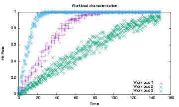
Static response of the cache.

c) Sampling the output: We also need a categorization of the statistical process within the system, that is to understand the process, sometimes this is known as workload characterization.

In this system to be controlled is the cache size, i.e. the number of items to hold is n. The cache operates an LRU policy (oldest evicted) in this work. Assume we want the cache to maintain a hit ratio of 70%. The output variable is a cache hit or miss, a boolean (a Bernoulli trial), therefore maintain the average number of successes over the k most recent requests. The uncertainty in estimating the correct number of hits/missed is approximately

       +- 0.5

  $latex \frac{1}{2}$

A  =  ——–

     √ (k)

Some explanation is needed, the variance of a Bernoulli random variable is Y = p(1 − p). The reason is that the error in the estimate of the hits or misses can be either absolute Aˆ − A or relative (Aˆ − A)/A. The relative error rate (after some simple algebra) gives the relative accuracy of the naive estimator is determined by

\math{1}{sqrt(kp)}

1 

——

 √kp

which is the expected number of hits in k trials. In other words the relative accuracy measured by the standard deviation of the estimator normalized by the exact answer (A). From a control point of view the relative accuracy depends on the expected number of hits, not the number of samples which is important. Therefore if we want to control the hit rate to within ± 0.05 we would need k to be 100. That means before increasing or decreasing the cache size to within 0.5% one would need to sample 100 cache accesses. 

TABLE I. ESTIMATED PARAMETERS FOR GAUSSIAN, ZIPF AND THE ORANGE DATASET FROM K(1 ^{− e( − (t − τ)/T)})

Method	K	T	τ	λ
Gaussian
Zipf (α = 1)
Dataset

Table I summarizes the estimated parameters … Note: Include a small paragraph, otherwise integrate the subsection into the previous one.

D. Ziegler-Nichols

Tuning algorithms: In this section we focus on the particular tuning algorithms. The Ziegler-Nichols closed-loop tuning is widely known as an accurate heuristic method to determine settings of PID and PI controllers [4, 5]. It is used so often in the process industry, it is almost always used as a benchmarking technique when designing an analog controller. An essential part of Ziegler-Nichols tuning is that little knowledge of the plants transfer function is needed, one only needs to know the plants (caching in our case) step-input response. This is why the static and dynamic steps were done to ascertain the time constants.

Ziegler-Nichols is also useful for self-regulating processes which (eventually) reach a steady state in response to a disturbance. to a sudden setpoint change, in an open-loop configuration and without a controller is observed. The idea is to fit a tangent to the response curve to the impulse. τ and λ are estimated from the gradient and cross intersection point see [6, 7] for more details see “process reaction curve”.

A dataset and computing environment

Orange labs data

The dataset used within this paper is a 3G data set from Orange labs in France and was obtained as part of the EU project SAIL. The dataset comprises http requests taken over the whole country between the access network and backhaul network, an example of two records is shown below.

1. GET 200 Fri Dec 16 16:59:59 2011 692023bd141d3b4f 10.224.54.166 84.233.158.134 /RF_Live/Le_flux_OPML_de_France_Inter.xml app.radiofrance.fr text/xml 752 2c7700154d85a248

2. POST 200 Fri Dec 16 16:59:59 2011 bb3f3e76e0b7dfe9 10.222.63.222 64.151.73.102 / ocsp.digicert.com application/ocsp-response 1100 4f0815901f64b878

The 11 fields of the dataset, HttpReq type, the return code, the data and time, a hash of the IMEI, the local client IP address, the public IP address, the path on the server, the domain, the MIME type, the size in bytes and the hash of the base station ID. The total size of the requests are 5.7 TB split into 952 hourly files. The total number of users is in the order of millions. It was captured between the 16th of December 2011 and the 25th of January 2012, which is around 40 days and covers the Christmas and New Year’s periods. It contains around 54 billion requests, and the total amount of data requested is in the order of 6 × 10¹⁶ bytes, giving an average of around 2MB per request with a standard deviation of around 41 MB. For the first hour, the (reported) minimum object size being 0 bytes first quartile being 47 bytes, the median 537 bytes, the mean 469,509 bytes and the 3rd quartile 4863 bytes and the maximum 3.2 × 10⁹ bytes. A 16TB disk could hold 0.03% of the total data requested, and a 2TB disk could store around 600 maximally sized objects. Given the mean and median differ by so much, we can easily see the data is highly skewed and very variable over time, regarding size, which has implications for caching. Information on the dataset can be found in [8, 9, 10].

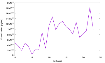
The time evolution of the dataset are shown in figure 6 and 7. In the weekly traces, two partial regional outages were observed (confirmed by the operator) whilst the daily trace clearly shows the 24 hour human cycle.

The two plots show the usage of the network over the 40 days, with dips at the weekend. The second over just one day to show the individual trends (day-night transitions).

Dataset (down)sampling for faster processing

The unadulterated raw dataset was 5.7TB on disk. Sampling the dataset allows the http requests to be held in memory and reduced the processing time, in our case, from about 24 hours to about 15-20 mins. This variation was due to the busy days and hours, as seen in figures 6 and 7. We made three downsampled versions from the original 5.7TB down to 82GB 45MB and 11MB which corresponds to 3.3%, 0.8% and of the original size. To derive the samples we used a technique known as reservoir sampling. It is from a family of randomized algorithms and chooses a subset of samples from a large(r) set. More formally, one selects k samples from a list of n items. In this case our k’s are 65K, 260K and 1M and our n is 3×10¹⁰. The algorithm by [11] essentially uses an array reservoir of (maximum) size. As an example, we wanted to see how many samples we would need to find statistically stable measures of the downsampled datasets, the average file size is shown in Figure 8.

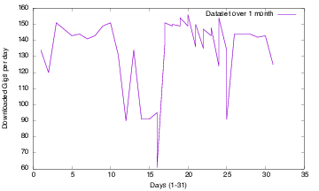
Fig 6. Data up and download volumes for the whole dataset per day (40 days).

Request analysis

Popularity and item size

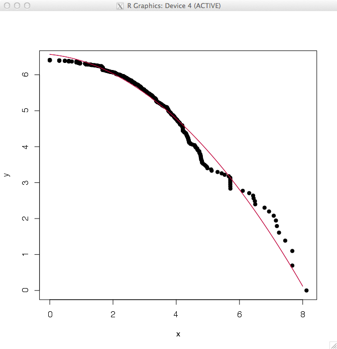
Popularity in terms of requests and volume is a key factor, as an example, the number of requests per hour, for the top 10 is as in Table II. This is an example of the dataset we had, and it also shows that it was collected and collated in France. From other studies, of this, and other datasets, the “top hitters” are somewhat uniform around the world. The distribution of the file sizes is shown in the CDF of figure 9, where the many small and significantly large files can be seen. This plot does not show all the 54 billion requests, but a small (around 1 million) fraction of all requests. Figure 10 shows a common log-log plot of the popularity (Y-axis) of the items against their rank (X-axis). This shows us how popular the items, independent of their size. A fit of the log-log plot, gives some intuitive idea of how skewed the power law fit it, a high value indicates there are only a few very popular unique requests (URL+Domain) are responsible for most of the requests, this is a steep fit on the log-log plot.

This is both true and false for this dataset, as the table II shows, some domains are very popular, however, depending on the cache size, many medium popular requests can be cached as well. Power-law or Zip parameters have been reported between (0.7 − 1.1] in the literature, so it is difficult to draw some conclusions, as the media type is important [12]. A lower power-law exponent means the popularity is more even across the catalog. A fit is shown in the figure, using 2 parameters, a curve fit to show some form of further analysis can be done directly related to caching, such as Che’s approximation [13] a remarkable relationship between the power law exponent and the hit rate of a LRU cache. 

Sampled mean size over time, showing after about 5000 samples we can reach a reasonable estimate of the mean, but using only 1-3% of the data. 

B. Time series analysis

Looking at the series of downloads (or requests) and analyzing them over time is worthwhile where the frequency of the event is known. In the case of accesses (or downloads) we have a clear cyclic trend, either over the day or week. Slightly weaker cases can be made for hourly trends or monthly. In Figure 11 we show some analysis of the original accesses in the top plot, the trend, cycles and random components in the figure. We do not use the information in the hand-tuned control algorithm, but will be future work. 

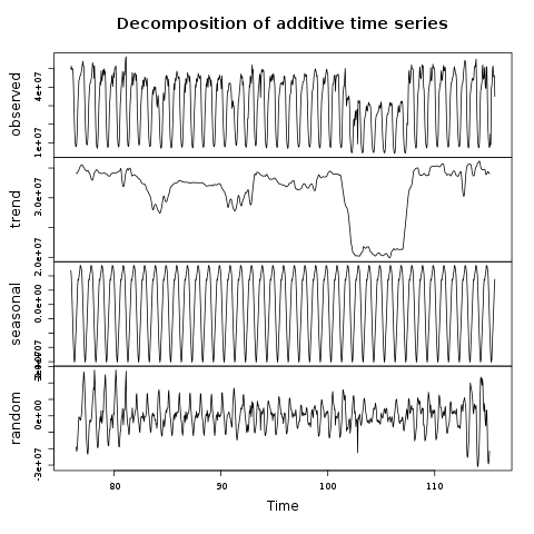
We can glean information from the time-series in the time responses of the system, as cyclic behaviors can be accounted for. The season and trend cycles can be removed from the observed behavior. The data request sizes can be provided more accurately by basically subtracting and taking the absolute value of the season and trend for the particular day and time. What is left is the truly random value as shown in the lower plot of figure 11. A time series approach has three extra benefits, firstly the residual requests are more likely to be Gaussian distributed, which gives easier to handle requests and less extreme values, and it also helps us set the parameters for the smoothing filter, essentially we can lessen our horizon for looking ahead, 100 in the case of 0.05% accuracy, can be reduced if needed. In other words the requests are more formed around a central value and variance, that is better treated for Gaussians.

A caching simulator

Code

We have chosen to simulate the hierarchical cache structure with a tree-based data structure written in C++. The use of a tree structure is natural for a hierarchy, and the use of a compiled object-oriented language such as C++ provides us with both speed and flexibility, for example derived classes (we use server and clients) and virtual functions for the eviction policies. The simulator comprises approximately 1500 lines. The server class has the capacity to hold all objects. Clients are leaf nodes that can initiate requests but cannot serve further, whilst caches can reply to, and pass onward, requests. Unlike the server, the intermediate caches have limited storage, so eventually they will fill and items will need to be evicted, on a one-by-one basis.

It is assumed that the total size of the objects stored at the server is greater than the total size of the cache memories, otherwise we could store all items. Our simulator can only emulate a hierarchical tree only at this moment, with several servers, but other topologies are not supported currently. We read or generate data for the client requests and in the trace case use it for initially populating the servers. Control is available for each cache however we show only the results for a single cache. Further work is being done on, multi level cache simulation with control, more details can be found in [2], [14].

The object-oriented programming style turns out to be conducive in building a simulator, as we can replace the caching visualization with alternative ideas. Using C++ and Emscripten we can take the object code from Saizu and convert to runnable code within a browser. Furthermore, with the addition of a small library (PicoJSON) it is possible to change the input parameters and single step the simulator within the browser for a good understanding of the dynamics. With this feature we can verify the cache static dynamics as shown in figure 5.

Visualization

Given the complexities, dimensions and dynamics, one result we will present is visualization of the implemented control and caching. Saizu shows the dynamics of the caches, on an individual case and within the hierarchy. The visualization tool, built from Javascript. We have three different views, depending on the needs of the experimenter. The visualization takes a request from either the Zipf-law distributed data or a request from the Orange dataset and allocates each request to one of the bottom caches, typically a 3G base station. In a fixed Internet scenario each request could form a DSLAM. If the item is in the cache it is served back to the requester. If not, the next cache up the tree, an operator cache for example is searched, again if found, it is served back down the tree.

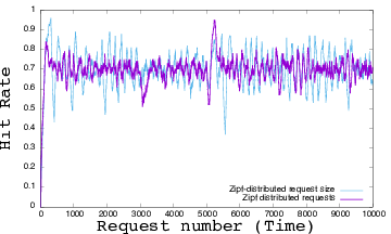
The process continues up the tree until the item is found or retrieved from the original server. The illustration shows how the caches fill from an unpopulated system, but over time only the popular items will remain stored. Moving the mouse over will show which items are in each cache (not shown in illustration). We have seen at an off-peak 45 ± 20 http requests per base station, and up to 200 ± 75 for busy hour periods. Note this is http, not TCP or IP packets. We believe an in-memory PI controller could easily handle this rate, and would be pretty straightforward to implement in hardware. From SIMULINK to hardware interfaces are available, with ARM support for example. This approach alleviates custom chip design and allows updates to be done in software. With a relative naive approach, we have shown that a variance reduction can be reduced by 30%. To show the difference of a real workload characterisation we show a Ziegler-Nichols PI control plus smoothing for Zipf distributed and real dataset workloads. A ZN controller is simple and has a wide utilization in industry. 

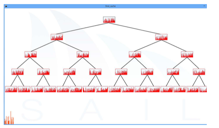
Figure 15 shows the stabilization of a cache with respect to the cache hit ratio. The hit rate shown in with higher variance is from the Zipf distributed requests while the lower variance plot is from using the Orange-based trace data characterizing the workload. In the figure above, the mean of the Ziegler-Nichols was 69.9% ± 9.2 %, whilst the mean from our system identification approach was 69.8% ± 6.4% which is around a 30% reduction in the standard deviation. Still, the cache fills, and we need to evict items, in this study we use the Least Recently Used (LRU) policy, but it is natural to compare this with others, particularly LFU and RND (Random). We also believe we can reduce the standard deviation (the square root of the variance) of the hit rate with a more sophisticated workload characterization. We implemented a control algorithm with the help of a Python control package [15]. 

Related work

Lu et al. look at proxy caching differentiated caching services using a control theoretical approach [3]. They evaluate a Proportional-Integral-Differential (PID) controller in Squid, and show that a differentiated caching service provides better performance for their (so called) premium content classes. Their work is similar to ours in the sense that they use a control theoretic approach, but differs in that they look at a two service level model and caching “first loaded” pages, e.g. index.html whilst we look at a single service level and audiovisual content. [3] look at performance differentiation for web access. More specifically, proxy caching differentiated caching services using a control theoretical approach. They evaluate a PID controller in Squid, and show that a differentiated caching service provides better performance to the premium content classes. [16] show the benefits of formal feedback-control design. They argue that control theory provides a powerful framework that simplifies the task of designing an adaptive system. Open-loop adaptation, they argue, is vulnerable to unpredictable behaviors with unknown or statistically complex workloads, especially when not considered at design time. We have given one example where one such case might be appropriate, but more research needs to be done on the input, often called system identification.

Ben Abdesslem et al. [10], analyze the same dataset and extract video requests by mobile users to a popular video streaming website. Their analysis shows that depending on the cache size and algorithm parameters, up to 20.33% of the requests can be served by a local cache. Their work is similar to ours in that they look at the cacheability of video from the same dataset, but differs in that we consider all video MIME types, audio too and we look at the dynamic sizing of cache(s).

Imbrenda et al. [17], look at the use of micro CDNs in ISP access and backhaul networks to reduce redundant web traffic. With a micro CDN they refer to a content delivery system composed of (i) a high speed caching substrate, (ii) a content based routing protocol and (iii) a set of data transfer mechanisms made available by content-centric networking. They use the same data set as we did, and characterized popularity and request cacheability, to infer potential traffic reduction enabled by micro CDNs. Methodologically somewhat related to our approach are also other network trace-driven media content caching studies – see, e.g., [18], [19]. For example, the analysis presented in [18] provided previously seminal insights into video streaming demands in cellular networks. In [19], the authors evaluate the gain in cache efficiency introduced by web caching and TCP-based redundancy elimination approaches.

Focusing on the Quality of Experience (QoE) of video delivery, several approaches adapt the bit rates offered by caches to the clients’ needs [20], [21]. For example, in [20], the authors tackle the problem of player-triggered switching between different encoding bitrates which has been observed in cellular network traces. Since this phenomenon has an effect on both QoE and caching, they propose a control theoretic approach, promoting specific bitrates, which improves the cache hit-ratio while also increasing the player stability. Other cache policies ARC (Adaptive Replacement Cache), GDSF (Greedy-Dual Size Frequency) and LFU + Dynamic Lifespan, LRR (Least request rate) are relevant, as it is not clear, which replacement policy would inter- operate best with the Saizu, see [22] for a survey on caching, albeit published in 1999, with the same author publishing caching for content distribution in 2013 [23].

Beyond using network traces, insights for predicting which audiovisual content needs to be cached can be derived by correlating topics popular in social media versus video download statistics, e.g., see [24]. [25] look at a unified approach to the performance analysis of caching. They propose a unified methodology to analyze the performance of caches (both isolated and interconnected),by extending and generalizing a decoupling technique originally known as Che’s approximation, which provides very accurate results at low computational cost. They consider several caching policies,taking into account the effects of temporal locality. In the case of interconnected caches, their approach allows us to do better than the Poisson approximation commonly adopted in prior work. Their results, validated against simulations and trace-driven experiments, provide interesting insights into the performance of caching systems.

Discussion

In this work, there are many things we need to bring to a discussion, as there are some tradeoffs in this work, like many engineering approaches. These are the QoE factors, the controller choice and implementation considerations. We begin with the chain of reasoning in Saizu: buffering events (Quality of experience) → Network measures (on path caching) → Cache performance (hit rate) → Stabilization (control theory) → Data analysis (Work characterization) → Audiovisual focus (database design) → Statistical dependency (Correlation analysis) → Trend behavior (Time series analysis) → Data reduction (Downsize sampling) → Fast database extraction (R + Data Table). Note: This list looks like unfinished text to the reviewers.

A. QoE

If we focus on video files, a small subsection of the audio video types, accounts for about 10% of the accesses, which is not large compared to the fixed network, but we know this is increasing, and the dataset is from late 2011. We assume that most of these accesses are from USB dongles. Of course there is some cost in complexity, however, it may well be worth introducing for better end-user quality of experience (QoE).

A cache cannot hold the 60 petabytes, therefore it may be better to fix a hit rate and to stabilize the hit rate. If buffers adapt for faster startup times or fast-forwarding, then the result of a miss will not impact the buffering scheme as much with an elastic cache. We have shown an initial research effort to regulate the cache size to stabilize the hit rate. 

B. The use of control theory

Feed-forward is one alternative in the control architecture. The stabilization may be better, as large, sudden disturbances, cause instabilities in the error term, which is the difference between observed and desired hot rates. If the disturbances are large, they may take time to propagate through the system. One can plan in feedforward situations for predictable load changes, such as lunch or evening high traffic demands. A simple engineering solution in this would be to put the popular, but large items in the static CDN content show in figure 2.

We have not used a differential term in Saizu. This was not a matter of principle, but mainly due to the noise, fluctuations from the varied, or skewed, or fast moving changes in the sizes and popularity of the requests. Although this is important in many Internetworking situations, queue length control, DoS attacks, it less likely to be used a CDN-like cache controller. That said, it has potential to be used as small scale predictor of the request pattern. For example, if the tracking error is positive, we know that the tracking error is increasing, so could apply a corrective action right away, even if the error is not (yet) significant. Fine controller tuning is something we will look at. There is an additional reason in this work, particularly, that is we will consider a hierarchy of caches in the longer term and the effect of control on one cache will propagate, and this is as yet, not understood.

Overshoot and undershoot of the desired value (70%) in control systems are common. A policy for dealing with following the output variable in control systems is usually left to the application. That is because, the cache operator would decide how aggressively to follow the desired hit rate. More smoothing will result in less changes to the actuator and closer following typically implies more changes to the input variable, the aggressive case. In many systems, changes to the actuator cost money, traditional control systems heat a substance, open a pipe, this usually has a cost, therefore the application should decide how closely to follow the output. In our work in caching, actuator costs also imply cost changes, more for a larger cost and less for a smaller one, given a hit rate that we want to set. The hit rate in itself may well be decided by an application for us too, the latency.

Time sampling, in this study we used an internal clocking mechanism, which means, for each request we calculate the hitrate, add a 1 or 0 to the hit counter and then check if it is over or under the desired rate. That is the system is “clocked” by the requests, or synchronous mode. An asynchronous mode is possible too, where the requests and control act independently.

C. Engineering considerations

On a practical note the small files (10 Kb or less) are usually not worth caching, as the overhead in accessing them, is too large in relation with the size retrieved. In contrast large files (10 Mb or more) are also not worth storing, as if they are popular, they will fill the cache quickly, making caching an expensive solution for these small numbers of files, that is to store a few popular files. These are probably better disseminated in a CDN (as Apple, Microsoft do) as a push-based dissemination model.

To put into context the hardware we had available we used a 2 CPU, 8 core machine at 3 Ghz with 128GB of physical memory and over 10TB of disk storage. The operating system was FreeBSD 9.1 using ZFS. We calculated we could use around 75% of the physical memory for processing, which means a total file size of around 80 GB. Given each hour is held as one file, of around 9 GB, we can hold about 9 hours of data in memory, without undue memory pressure. We found the I/O system was more vulnerable and unstable reading and writing such large files, therefore we tried to downsize files to around 40 GB.

Stability and disturbances, when feedback controlled systems experience large changes, it may be beneficial by adding the control of the feedback loop with a feed-forward control strategy. This is because feedback reacts to an error, the difference between the setpoint and the actual process output. If the disturbances, in our case, file sizes, are large and sudden, then waiting for the error to propagate through the loop could cause loop instability. A simple engineering solution to this is to filter small and, particularly large files, as storing these is financially uneconomical.

Energy concerns

Obtaining representative workloads as well as real values from hardware is challenging, either resorting to paper specifications. Getting real  data to generate realistic workloads is also troublesome to 1) build a system, 2) make it representative 3) measure its energy efficiency. In this work we have recreated a hardware “mini-system”, the cache represented by a single card UNIX based computer, such as a Raspberry Pi, Banana Pi or Odroid SoC systems. The clients, also will be single board computers, probably 2-5 units connected on a local network. Effectively they will be workload generators, the server will be a micro-ATX board computer, with low power use.

Future directions in caching

Control

Within this work we have also dedicated some space to the discussion, as there are numerous design decisions to be made. Also we have shown where future work could head, one direction in classical analog control or to a more modern state space approach. The simulator (FMDCache) and Javascript together Saizu are available from a public repository.

We have shown an initial research effort to regulate the cache size to stabilize the hit rate. The details of the control mechanism have not been given here, however it is a simple proportional-integral- derivative controller. The data is trace driven, but over a period of a few minutes only, we should of course run the workload over a longer period. The step sizes of the cache should be increased or decreased in units of disk/block size, which we currently do not, we assume any size adjustment. Somewhat further ahead in the research agenda, would be a multiple input/output controller. That said, one should be careful with inputs that are correlated in this case.

In this work, we used a transformation from time to the frequency domain, so called classic control theory. If we were to use more than one input, but keep a single output then we would look at multiple input and single output (or more) then we would need a more modern approach. Rather being based on a Laplace transform, we would use a linear system of nth order equations written in a coupled manner:

x[k + 1] = Ax[k] + Bu[k] + w[k] (2) y[k] = Cx[k] + v[k]

Where w[k] is the process noise and v[k] is the measurement noise. It is possible to solve equations 2 and 3, with solutions:

x[k + 1] = (A − BKC)x[k] + Br

Equation 4 determines the dynamics of the closed-loop system, actually the eigenvalues of the matrix are the modes of the dynamical system. We will look at this in the future, so as to go to to a MIMO solution as well as being able the machinery of linear algebra.

Conclusions

We have shown a standardized control theoretic approach of how to stabilize a cache hit ratio, populated with real data from a 3G network. In principle, without a feedback-like solution this is a difficult problem, as the system dynamics make the problem difficult. With the addition of some complexity within the cache and the remit of having some storage flexibility, we can control the performance of the cache dynamics. The results provide important indicators of behavioral patterns, caused by the user requests, in terms of placement and sizing. An application knows on average it will get a cache miss of the time and deal with it, in its unique way. Quality of experience is highly related to quality of expectation and applications that can handle uncertainty will yield better quality for its users. The solution of a C++ simulation engine and Javascript front end allow experimentation, in a browser and step by step to observe the dynamics.

---

Network and hit rates

Social media

Can cause huge fluctuations in demand patterns.

Spatial (topology) issues

Temporary items.

Data types and correlated

Language dependence

Network location

The type of users

Fixed or stationary users

Effect of network load, balance between local plus network delay and CDNs, so called coupled systems.

Network: Fan in and out

Cache size as a ration of catalog size.

Policies

Classic: LRU, LFU, RN

Modern: DARC, LRR

Content type

Apps (Fehmi)

TV  (Henrik)

Che formula

References

[1]  B. Bjurling and P. Kreuger, “Performance of cache placement policies,” in 10th Swedish National Computer Networking Workshop, SNCNW, 2014.

[2]  I. Marsh, “Elastic network resources: controlled caching,” in 10th Swedish National Computer Networking Workshop, SNCNW, 2014.

[3]  Y. Lu, A. Saxena, and T. Abdelzaher, “Differentiated caching services; a control-theoretical approach,” in Int. Conf. on Distributed Computing Systems, Apr 2001, pp. 615–622.

[4]  J. G. Ziegler and N. B. Nichols, “Optimum Settings for Automatic Controllers,” Transactions of ASME, vol. 64, pp. 759–768, 1942.

[5]  J. L. Hellerstein, Y. Diao, S. Parekh, and D. M. Tilbury, Feedback Control of Computing Systems. John Wiley & Sons, 2004.

[6]  K. Ogata, Modern Control Engineering, 4th ed. Upper Saddle River, NJ, USA: Prentice Hall PTR, 2001.

[7]  G. F. Franklin, D. J. Powell, and A. Emami-Naeini, Feedback Control of Dynamic Systems, 4th ed. Upper Saddle River, NJ, USA: Prentice Hall PTR, 2001.

[8]  F. Ben Abdesslem and A. Lindgren, “The Pursuit of ’ Appiness: Exploring Android Market Download Behaviour in a Nationwide Cellular Network,” in 5th International Workshop on Traffic Analysis and Characterization (TRAC), 2014.

[9]  Fehmi Ben Abdesslem, Anders Lindgren, “Large Scale Characterisation of YouTube Requests in a Cellular Network,” in IEEE WoWMoM, 2014, link.

[10]  Fehmi Ben Abdesslem, Anders Lindgren, “Cacheability of youtube videos in cellular networks,” in 4th workshop on All things cellular: operations, applications, & challenges. ACM, 2014, pp. 53–58.

[11]  J. S. Vitter, “Random sampling with a reservoir,” ACM Trans. Math. Softw., vol. 11, no. 1, pp. 37–57, Mar. 1985.

[12]  C. Fricker, P. Robert, and J. Roberts, “A versatile and accurate approximation for lru cache performance,” in 24th International Teletraffic Congress, ser. ITC. International Teletraffic Congress, 2012, pp. 8:1–8:8.

[13]  H. Che, Y. Tung, and Z. Wang, “Hierarchical web caching systems: modeling, design and experimental results,” Selected Areas in Communications, IEEE Journal on, vol. 20, no. 7, pp. 1305–1314, Sep 2002.

[14]  I. Marsh and A. Gunnar, “Hierarchical caching simulation with visualisation,” in 15th International Conference on Computer Modelling and Simulation, UKSim 2013, Cambridge, United Kingdom, April 10-12, 2013, D. Al-Dabass, A. Orsoni, J. Yunus, R. Cant, and Z. Ibrahim, Eds. IEEE, 2013, pp. 622–627. [Online]. Available: http://dx.doi.org/10.1109/UKSim.2013.154

[15]  J. Goppert, “Python control system library,” https://github.com/jgoppert/python-control, May 2014.

[16]  S. Velusamy, K. Sankaranarayanan, D. Parikh, T. Abdelzaher, and K. Skadron, “Adaptive cache decay using formal feedback control,” in Workshop on Memory Performance Issues, 2002.

[17]  C. Imbrenda, L. Muscariello, and D. Rossi, “Analyzing cacheable traffic in isp access networks for micro cdn applications via content-centric networking,” in Int. Conf. on Information-centric Networking, ser. INC. New York, NY, USA: ACM, 2014, pp. 57–66.

[18]  J. Erman, A. Gerber, K. K. Ramadrishnan, S. Sen, and O. Spatscheck, “Over the Top Video: The Gorilla in Cellular Networks,” in ACM SIGCOMM Conference on Internet Measurement Conference, ser. IMC. New York, NY, USA: ACM, 2011, pp. 127–136.

[19]  S. Woo, E. Jeong, S. Park, J. Lee, S. Ihm, and K. Park, “Comparison of Caching Strategies in Modern Cellular Backhaul Networks,” in Int. Conf. on Mobile Systems, Applications, and Services, ser. MobiSys. New York, NY, USA: ACM, 2013, pp. 319–332.

[20]  Z. Aouini, M. T. Diallo, A. Gouta, A.-M. Kermarrec, and Y. Lelouedec, “Improving Caching Efficiency and Quality of Experience with CF-Dash,” in Network and Operating System Support on Digital Audio and Video Workshop, ser. NOSSDAV. ACM, 2014.

[21]  D. H. Lee, C. Dovrolis, and A. C. Begen, “Caching in HTTP Adaptive Streaming: Friend or Foe?” in Network and Operating System Support on Digital Audio and Video Workshop, ser. NOSSDAV. ACM, 2014.

[22]  J. Wang, “A survey of web caching schemes for the internet,” SIGCOMM Comput. Commun. Rev., vol. 29, no. 5, pp. 36–46, Oct. 1999. Available: http://doi.acm.org/10.1145/505696.505701

[23]  J. Zhang, “A literature survey of cooperative caching in content distribution networks,” CoRR, vol. abs/1210.0071, 2012. [Online]. Available: http://arxiv.org/abs/1210.0071 

[24] A. Lobzhanidze and W. Zeng, “Proactive caching of online video by mining mainstream media,” in IEEE International Conference on Multimedia and Expo (ICME), July 2013, pp. 1–6.

[25] V. Martina, M. Garetto, and E. Leonardi, “A unified approach to the performance analysis of caching systems,” CoRR, vol. abs/1307.6702, 2013. Available: http://arxiv.org/abs/1307.6702 

[26] Cisco Visual Networking Index: Forecast and Methodology, 2013-2018.

[27] Manxing Li, Braun, Torsten; Trinh, Tuan Anh. Energy Efficiency Issues in Information-Centric Networking. Pierson, Jean-Marc; Da Costa, Georges; Dittmann, Lars (eds.) Energy Efficiency in Large Scale Distributed Systems: COST IC0804 European Conference, EE-LSDS 2013 Vienna, Austria.

[28] Athanasios V. Vasilakos, Zhe Li, Gwendal Simon, Wei You, Information centric network: Research challenges and opportunities, Journal of Network and Computer Applications, Volume 52, June 2015.

[29] Choi N, Guan K, Kilper DC, Atkinson G. In-network caching effect on optimal energy consumption in content-centric networking. In: IEEE ICC next generation networking symposium; 2012

[30] Guan K, Atkinson G, Kilper DC, Gulsen E. On the energy efficiency of content delivery architectures. In: IEEE ICC green communications workshop, 2011.

[31] Hasegawa, Y. Nakai, K. Ohsugi, J. Takemasa, Y. Koizumi and I. Paras, Empirically Modeling How a Multicore Software ICN Router and an ICN Network Consume Power, in Proceedings of 1st ACM Conference on Information-Centric Networking (ICN-2014), 24-26 September 2014. Paper

[32] The Art of Computer Systems Performance Analysis: Techniques for Experimental Design, Measurement, Simulation, and Modeling 1st Edition, http://www.amazon.com/The-Computer-Systems-Performance-Analysis/dp/0471503363

[33] Saizu: Cache hit stabilization of a real dataset using a control theoretic approach

[34] Ian, Andrea, Nima, Rickard, Anna, Johan, Daniel (Andreas)

Acknowledgment

This work was carried out during the tenure of an ERCIM Alain Bensoussan fellowship Programme for both Andrea Hess and Nima Dokoohaki, for Ian Marsh was financed by the KK-Stiftelsen project ”Forskningsmiljo for Internet med lag fordrojning” (READY), Diarenummer 20130086.

Net neutrality

Do we transfer all bits the same? We should.