
%
% Communication with vehicular networks: a traffic flow analysis
%
% \documentclass[conference, a4paper]{}
\begin{document}
%
% Title
%
Fluid flow models are used to study the interaction of vehicles on existing (and planned) road infrastructure in order to optimize flow through cities, towns and highways. The studies are often subject to a number of criteria such as acceptable journey times, $C_{O2}$ emissions and so on. In this example we are concerned with density, speed and vehicular density models.
Macroscopic fluid traffic flow models can be used to investigate queue buildups. This work is a theoretical (and numerical) example using scalar non-linear physical models to quantify variations in traffic conditions (density, speed, flux). These pages exemplify the theory using four common road phenomena, a long road stretch, traffic lights, junctions and a roundabout.
\section{Background}
Density fluctuations directly effect traffic characteristics. A further motivation for taking a macroscopic approach is to find the relationship between density, flux and velocity of vehicles en masse, a so called macroscopic approach. Much research is dedicated to how clusters of vehicles form and disperse.
In the first part of this post we give an introduction to the theory of traffic flow assuming non-familiarity of the reader. We begin with a single lane (scalar) linear traffic flow model and derive the conservation law. After introducing average vehicle velocity into the picture we present a non-linear model as introduced by Lighthill and Whitham in the 1950s. We then present a solution to this equation using the theory of characteristics and give an example. Shock and rarefaction waves, which can result in all wave equations, are presented and we show how to solve them and their significance in vehicular distributions.
We show techniques for solving them using so called jump and entropy conditions. In the second part we give some examples of the application of the previous section, in familiar road situations such as junctions. There is a short section on numerical methods, particularly robust ones, which uses the ideas presente.
In the final part of this page we present some simple simulations and a real study to show how the techniques map to the real world.
% ====================================================================
% Traffic flow model
% ====================================================================
\section{A traffic flow model}
\subsection{Velocity fields}
In the study of waves so-called $xt$ (position, time) plots are used which show the relation of the waves in space and time. Velocities from lines or curves on the $xt$ plots can be inferred. Choosing distance ($x$) for the $y$-axis and time ($t$) for the $x$-axis permits us to draw lines which indicate the velocity. Therefore the velocity at a particular time and position denoted $u(x, t)$ known as the velocity field:
\[
\frac{dx}{dt} = u(x, t) \quad \mbox{with} \quad x(0) = x_0
\]
In traffic flow illustrations it is quite common to reverse the axis with time $t$ on the $y$ axis and distance on the $x$ axis making the velocity the reciprocal of the gradient. characteristic equations which are one method of solving PDEs (see section \ref{sec:characteristics}) are clearer in this orientation. In this post we will usually show the traffic density on 2-D plots projected from a three dimensional space comprising position, time and traffic density.
In the figure above a simplified road model is shown $x_n$ are the positions of the vehicles, with length $L$ and separation $d$. %% If the average length of a vehicle is defined as $L$ then cars will be required to come to a halt if $\rho_{max} < 1/L$. $\rho_{max}$ is the number of cars when the traffic is bumper to bumper, i.e. the maximum. In the differential form above the derivative is always decreasing, i.e. it is $<0$. Later we will see density changes for a varying flows into the road segment as well as where stoppages can occur the static density is:
\[
\rho = \frac{1}{L + d}
\]
Now we will build up a simple model for the traffic flux from first principles (refer to the table below).
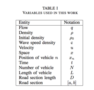
Let $\rho$ be the density of vehicles, the number at a fixed point (or interval) given by $\rho(x, t)$. $q$ is the flux of vehicles, the number passing a fixed point in unit time and is given by $q(x, t)$. A positive value of $q(x, t)$ indicates the flux is in the direction of increasing $x$, while a negative value of $q(x, t)$ indicates the flux is in the direction of decreasing $x$. $N$ is the number of vehicles on the road segment under consideration. Initially we will assume that no cars enter or leave the road section, thus we conserve the number of cars in that interval. The flux, density and velocity of the vehicles are related by the important relationship, remember the quantities are always functions of location and time:
\[
q = \rho \cdot u, \quad \mbox{OR} \quad q(x, t) = \rho(x, t) \cdot u(x, t)
\]
% —————————————————————-
% A (linear) conservation law
% —————————————————————-
\subsection{A linear conservation law}
We now consider the number of vehicles ($N$) in a \textsl{road
segment} $[a, b]$ given by:
\begin{equation}
\label{int_traffic_density}
N = \int_a^b \rho(x, t)\,dx
\end{equation}
The integral of the traffic density. The number of cars between $a$ and $b$ may change due to the \{in} and \textsl{out} flows. We allow the number of cars crossing the boundaries $a$ and $b$ to be variable i.e. $q(a)$ and $q(b)$. The rate of change in the number of cars is given by:
\begin{equation}
\label{Rate_of_change}
\frac{dN}{dt} = q(a, b) – q(b, t)
\end{equation}
The quantity flowing \textsl{into} b therefore has a negative sign. It is possible to derive this result in another way: We would like to obtain the number of cars crossing $x = b$ between $t=t_0$ and $t=t_1$. Since $q(b, t)$ is the number of cars crossing at $x = b$ per unit time, then $\int^{t_1}_{t_0} q(b,t)dt$ is the number crossing at $x=b$ between $t=t_0$ and $t=t_1$ ($N(t_1) – N(t_0)$) is:
\[
\int^{t_1}_{t_0} q(a, t)dt – \int^{t_1}_{t_0} q(b, t)dt = \int^{t_1}_{t_0} q(a, t)dt – q(b, t)dt
\]
By dividing this expression by $t_1 – t_0$ and take the limit as $t_1$ $\to$ $t_0$. By combining \ref{int_traffic_density} and \ref{Rate_of_change} we obtain:
%
% Conservation law
%
\begin{equation}
\label{conservation_law}
\frac{d}{dt}\int^b_a \rho(x, t)dx = q(a, t) – q(b, t)
\end{equation}
The equation states that the change in the number of cars in the section is due \textsl{only} to the flux across the boundaries. No cars leave or enter the considered section. Equation \ref{conservation_law} is known as the \textsl{integral conservation law}. Taking limits over an infinite segment of road ($x \to \pm \infty$) and integrating the LHS of equation \ref{conservation_law} gives:
%
%
%
\[
\int^{\infty}_{-\infty} \rho(x, t)dx = \mbox{constant}
\]
which states the total number of cars is constant for all time. In order to determine the constant, we need to know the initial number of cars ($N_0$) or the initial density $p(x, 0)$. For a finite length ($a \le x \le b$) in the right hand side of \ref{Rate_of_change}:
\[
q(a, t) – q(b, t) = – \int^b_a \frac{\partial}{\partial x}[q(x, t)]dx
\]
Taking the derivative with respect to $b$ ($b = a + \triangle a$) dividing by $\triangle a$ and taking the limit as $\triangle a \to 0$ gives:
\[
\frac{\partial \rho(b,t)}{\partial t} = – \frac{\partial}{\partial b}(q(b,t))
\]
We can replace the $b$ by $x$ as it can be anywhere on the road, which results in:
\begin{equation}
\label{differential_form}
\frac{\partial \rho}{\partial t} + \frac{\partial q}{\partial x} = 0, \quad
\rho_t + q_x = 0
\end{equation}
which is the \textsl{differential} form of the conservation law, and assumes that $\rho$ and $q$ are continuous. Even when they are not, a solution may be found that is known as a \textsl{weak} solution. A weak solution is one that is satisfied by a function which may not be differentiable, not even continuous, only measurable and bounded. The equation expresses the fact that changes in the number of vehicles are only due to the flux across the boundary, if the right hand side is zero.
The number of vehicles in the region $[a, b]$ is \textbf{not} constant. If that were true, $q(a, t) = q(b, t)$ or $\frac{d}{dt} \int^b_a \rho(x, t)dx = 0$. Until now, the equation is linear and depends on only two variables, the position $x$ and the time $t$. The conservation equation is a single equation but with two unknowns, so we need an extra condition to solve it.
% ——————————————————————-
% A non-linear traffic flow equation
% ——————————————————————-
\subsection{A non-linear traffic flow equation}
It seems reasonable to expect the velocity to be a function of density in some way. One is the velocity to be monotonically decreasing with increasing density. The flux $q$ for a traffic flow problem could be of the form:
\begin{equation}
\label{flux}
q = q(\rho), \quad q(\rho) = \rho(1 – \rho)
\end{equation}
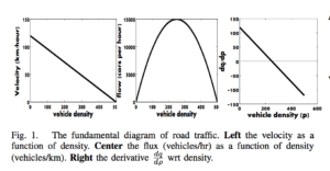
When the density is lowest ($\rho = 0$) the flux is zero, there are no vehicles to constitute a flow. Conversely, when the density is maximum ($\rho = \rho_{max}$) vehicles are queued up back to back, no movement and again no flow. For a quadratic relationship we have a convex function as shown in the plot below.
%
% Road traffic laws
%
%\begin{figure}[!h]
% \begin{minipage}{0.30\linewidth}
% \centering
% \epsfig{file=Images/flux-density.eps , height=3cm, width=3cm}
% \end{minipage}
%
% \begin{minipage}{0.30\linewidth}
% \centering
% \epsfig{file=Images/speed-density.eps, height=3cm, width=3cm}
% \end{minipage}
%
% \begin{minipage}{0.30\linewidth}
% \centering
% \epsfig{file=Images/dq-dq_versus_p.eps, height=3cm, width=3cm}
%\end{minipage}
% \caption{Left. The fundamental diagram of road traffic: the flux
% (cars/hr) as a function of density (cars/km) Middle. Velocity
% Vs. density Right. $\frac{dq}{d\rho}$ versus $\rho$}.
% \label{traffic_law_relations}
% \end{figure}
Going back to the differential conservation equation:
\[
\rho_t + q_x = 0
\]
Rewrite the change in flux as:
\begin{equation}
\label{eq:foo}
q_x = \frac{dq}{d\rho}\rho_x = \rho_t + (\frac{dq}{d\rho}) \cdot \rho_x = 0
\end{equation}
As an example if the flux depends on the density such as $q = \rho^2$
then
\[
\rho_t + (2 \rho) \cdot \rho_x = 0 \quad -\infty < x < \infty, \quad t > 0
\]
with the initial condition:
\[
\rho(x, 0) = \rho_0(x) \quad -\infty < x < \infty \] If the initial density is $\rho(x, 0) = \rho_0(x)$ then to find the density at some future time $t$ we would need to solve equation \ref{eq:foo} with the initial condition as well. For more intuition, in light traffic, the driver is relatively free to decide the velocity they wish. In heavier traffic, they encounter other vehicles and it is inevitable that the average velocity will be reduced. Therefore a simplifying assumption is the following: the velocity of the vehicles depends only on the density of the vehicles. This is known as \textsl{local density} condition. Note that the relation between flux and density will depend on weather, road conditions \cite{weather}, speed limits and so on.
Flow example
Optimizing such a function for density is trivial. However for more complex functions, it may not be straightforward. We will return to this topic later. But, next we want to introduce the concept of vehicle \textsl{velocity} into the differential form of the conservation equation: % % including vehicle density % \subsection{Introducing the vehicle velocity} Another way to view the flux ($q$) is the product of the density ($\rho$) and the velocity ($u$), as we said earlier: \[ q = \rho \cdot u \] Substituting the above relationship into the conservation equation we obtain: \[ \frac{\partial \rho}{\partial t} + \frac{\partial }{\partial x}(\rho u) = 0 \] or, considering that the velocity is a function of the density: \[ \frac{\partial \rho}{\partial t} + \frac{\partial }{\partial x}(\rho u(\rho)) = 0 \] moreover by the chain rule: \[ \frac{\partial \rho}{\partial t} + \frac{\partial q }{\partial \rho} \frac{\partial \rho}{\partial x} = 0 \] Density waves are important, as they describe how changes in the velocity of vehicles propagate through lines of traffic as shown in the New Scientist video\footnote{http://www.youtube.com/watch?v=Suugn-p5C1M}. The propagation speed is denoted $c$ which is equal to $\frac{dq}{dt}$ for the density waves carrying changes of density through streams of cars in a single lane. If the mean velocity of cars \textsl{decreases} with increasing density:
% % Relating density wave speed and car speed % \begin{equation} \label{c} c = \frac{dq}{d\rho} = \frac{d}{d\rho}(\rho u) = u + \rho\frac{du}{d\rho} \end{equation} % % % \begin{equation} \label{c_u} c \le u \quad \mbox{only if} \quad \frac{du}{d\rho} \le 0 \end{equation} and $c=u$ only at very low density (from equation \ref{c}). Which means the speed of the shockwaves is always less than the mean speed of the vehicles themselves. The ramifications of this is that drivers always react to changes in density \textsl{ahead} of their current position and not behind. Cars in a congested region have larger density around them and consequently must slow down. The cars behind travel faster than in the congested region, and they then move into the higher density region, but slow down before they reach the congested region. The speed of the density waves we have been discussing is $\frac{dq}{dt}$ it can be found from the fundamental diagram of road traffic, figure \ref{traffic_law_relations}, from the gradient at the point $u = q/\rho$.
\section{Characteristics}
This section describes one method to solve the differential equations. The method is very useful for us to ascertain when certain physical road changes are taking place, such as vehicles spreading out in distance (and over time) as well as compressing. The method of characteristics is one technique for solving hyperbolic PDEs. Typically, it applies to first-order equations only, although this includes non-linear forms, which we will require. The general method is to reduce a PDE to a family of ordinary differential equations (ODE) along which the solution can be found from some initial data given on a suitable hypersurface. In linear situations the characteristics will be parallel straight lines (solutions to 1st order differential equations), in non-linear cases the lines may not be parallel (but straight). The method of characteristics can be thought of finding a a solution along a hypersurface which is projected ahead in time. Some works even say “information” is propagated ahead in time. % % Characteristics and shocks model
% %\begin{figure}[ht] % \begin{minipage}[b]{0.3\linewidth} % \centering % \epsfig{file=Images/characteristics-old.eps, height=3cm, width=3cm} % \end{minipage} % \begin{minipage}[b]{0.3\linewidth} % \centering % \epsfig{file=Images/characteristics.eps, height=3cm, width=3cm} % \end{minipage} % \begin{minipage}[b]{0.3\linewidth} % \centering % \epsfig{file=Images/shock.eps, height=3cm, width=3cm} % \end{minipage} % \caption{Characteristics and shock wave solutions} % \label{characteristics} % \end{figure}
The `curves` are parallel lines in the $xt$-plane with gradient $1/c$ but starting at different points $(x_0, 0)$ on the x-axis see figure \ref{characteristics}. The derivative $\frac{dx}{dt}$ is the velocity of the characteristics, which we will denote $c$, which has units of velocity, and is sometimes called the characteristic velocity. From the conservation law we can construct the value of $\rho(x,t)$ at any point $(x, t)$. From the point (x,t) it is possible to extend the line back to the x-axis. Using the substitution $\rho_0 = x – ct$: \[ \rho(x, t) = \rho(x_0, 0) = \rho_0(x_0) = \rho_0(x – ct) \] The special curve $(x(t),t)$ starting at the point $(\rho_0, 0)$ is determined by the conditions: \[ \frac{dx}{dt} = c, \quad x(0) = x_0 \] Solving the IVP shows that x(t) is given by: \[ x = ct + x_0 \] which is called the characteristic or \textsl{characteristic curve} of $\rho_t + c\rho_x = 0$. The initial condition gives the profile at time $t = 0$. For later points in time $t > 0$, $x(t), t$ is a curve in the xt-plane. As $(x(t), t)$ moves along the curve, the value of $\rho(x(t),t)$ changes at the rate of (chain rule):
\begin{equation}
\frac{d}{dt}\rho(x(t), t) = \rho_x(x(t), t)\frac{dx}{dt} + \rho_t(x(t), t)
\end{equation}
The RHS $\rho_t + \frac{dx}{dt}\rho_x$ resembles the $\rho_t +
c\rho_x$ part of the conservation law. If we select the curve $(x(t),
t)$ so that:
\[
\frac{dx}{dt} = c, \quad \frac{d}{dt}\rho(x(t), t) = \rho_t(x(t), t) + c\rho_x(x(t), t)=0
\]
which implies the value of $\rho$ is constant long the curve. so the value of each point on the curve is the same as the initial point $(\rho_0, 0)$. As an example consider the following conservation law:
\[
\rho_t + 4\rho_x = 0, \quad -\infty < x < \infty, t > 0
\]
\[
\rho(x, 0) = \mbox{arctan(x)}
\]
Along a curve $(x(t), t)$, the derivative of $\rho(x(t), t)$ is
\[
\frac{d}{dt}\rho(x(t), t) = \rho_x(x(t), t) \frac{dx}{dt} + \rho_t(x(t), t)
\]
Picking $x(t)$ to satisfy:
\[
\frac{dx}{dt} = 4, \quad x(0) = x_0
\]
so $\rho(x(t), t)$ has a constant value along $x = 4t + x_0$. At any point $(x, t)$ the characteristic line through this point extends back to $(x_0, 0)$ on the x-axis where $x_0 = x – 4t$. Since $\rho$ is constant \textsl{along this characteristic}, the value of $\rho$ at $(x, t)$ is:
\[
\rho(x, t) = \rho(x_0, 0) = \mbox{arctan}(x_0) = \mbox{arctan}(x – 4t)
\]
The solution of the IVP is a traveling wave with profile arctan(x) moving with velocity 4.
% ——————————————————————
% Shock and rarefaction waves
% ——————————————————————
\subsection{Shockwaves and rarefaction waves}
An important part of any wave approach is the formation of so called shockwaves (or jump-discontinuities) and rarefaction waves. Shockwaves are also known as traveling discontinuities. Rarefactions are continuous waves. In traffic situations they typically arise under braking or at junctions/roundabouts. The traffic compresses sending a density wave backwards. In rarefaction traffic fans out with increasing distance between the cars over time.
% —————————————————————
% Characteristics for shockwaves and rarefaction
% —————————————————————
%\begin{figure}[ht]
% \begin{minipage}[b]{0.49\linewidth}
% \centering
% \epsfig{file=Images/traffic-ic1.eps, height=4.9cm, width=4.9cm}
% \label{fig:ic1}
% \end{minipage}
% \begin{minipage}[b]{0.49\linewidth}
% \centering
% \epsfig{file=Images/traffic-ic2.eps, height=4.9cm, width=4.9cm}
% \label{fig:ic2}
% \end{minipage}
% \caption{Rarefaction and shock characteristics}
% \label{rare-shock}
% \end{figure}
In traffic flow theory they can form where there is a jump in the density at a given place and time $x_s(t)$. Technically a function $f(x)$ has a jump-discontinuity at $x=x_s$ if the limit from the right of $f(x), f(x_x^+)$ does not equal the limit from the left $f(x_x^-)$, but both limits exist. The method of characteristics can construct a solution but only up to the point where the function becomes multi-valued, which pictorially is where characteristic lines intersect, see figure \ref{rare-shock}.
% ———————————————————————-
% Time to shock
% ———————————————————————-
\subsection{Time to first shock}
The time where the characteristics first cross, called the time to shock or the earliest shock can be interpreted as the time when the braking must occur on a road segment. We call this time $t_b$ and need to find when $\rho_x$ becomes infinite.
\[
\rho_t + c(\rho)\rho_x = 0, \rho(x,0) = \rho_o(x) \quad -\infty < x < \infty, t> 0
\]
at the point $(x,t$) is $\rho_0(x_0)$ where $x_0 = x_0(x,t)$ determines the starting point $(x_0, 0)$ of the characteristic passing through $(x,t)$. The derivative $u_x$ is
\[
\rho_x(x, t) = \rho_0′(x_0)\frac{\partial x_0}{\partial x}
\]
by the chain rule. The value of $x_0$ defines the starting point $(x_0, 0)$ of the characteristic through $(x,t)$ and is defined by the implicit equation:
\[
x = c(\rho_0(x_0))t + x_0
\]
After taking the derivative using implicit differentiation and taking the partial derivative wrt $x$ gives the left equation. The braking time can be found by considering when the denominator becomes zero, which means considering each part in turn, after some algebra we obtain the right equation.
\[
\frac{\partial x_0}{\partial x} = \frac{1}{1 + t\frac{d}{dx_0}c(\rho_0(x_0))}, \quad t_b = \frac{1}{\frac{d}{dx_0}c(\rho_0(x_0))}
\]
% ———————————————————————-
% Rankine-Hugoniot jump conditions
% ———————————————————————-
\subsection{The Rankine-Hugoniot jump condition}
Hyperbolic conservation laws can develop discontinuities, even when provided with continuous initial data. We would like to know how a discontinuity propagates when formed, more specifically its speed. The Rankine-Hugoniot jump conditions relate to the behavior of shock waves traveling normal to the prevailing flow. The jump condition states that the jump in the flux across the discontinuity is equal to the jump in the density of the conserved quantity (in our case density) multiplied by the speed of the discontinuity. By considering $\rho(x, t)$ to be piecewise smooth (not necessarily continuous), it is possible to construct a solution. If $(x_s(t), t)$ is a curve in the $xt$-plane which separates the 1st quadrant into two parts shown in the middle and right illustrations of figure \ref{characteristics}. Along the jump discontinuity $x_s$ is called the shock path (highlighted in the plot). The function $\rho(x,t)$ is a piecewise smooth solution of equation \ref{con} if $\rho(x,t)$ satisfies the two numbered properties below:
\begin{equation}
\label{con}
\rho_t + q_x = 0, \; -\infty < x < \infty, t > 0
\end{equation}
\[
\rho(x, 0) = \rho_0(x)
\]
1. $\rho(x,t)$ has continuous first derivatives $u_t$ and $u_x$ and satisfies the IVP in region $R^-$:
%
%
%
\begin{eqnarray*}
\rho_t + q_x &=& \mbox{for} \quad (x,t)\quad \mbox{in} \quad R^- \\
u(x, 0) &=& u_0(x) \quad \mbox{for} \quad x < x_s(0) \end{eqnarray*} and in region $R^+$ \begin{eqnarray*} \rho_t + q_x &=& \mbox{for} (x,t)\quad \mbox{in} \quad R^+ \\ u(x, 0) &=& u_0(x) \quad \mbox{for} \quad x > x_s(0)
\end{eqnarray*}
2. Also at each point $(x_0, t_0)$ on the curve $(x_s(t), t)$, the limit of $\rho(x,t)$ as $(x,t) \to (x_0,t_0)$ in $R^-$ and the limit of $\rho(x,t)$ as $(x,t) \to (x_0,t_0)$ in $R^+$ exist, but may not be equal. The general idea is to use $t_b$, the breakdown of the solution as the $t=0$, and to construct a curve through the crossing characteristics to separate the ones approaching from the left and the right. The conservation law can be used to select a single curve, despite many existing. Going back to the integral form:
\[
\frac{d}{dt}\int^b_a \rho(x, t)dx = q(a, t) – q(b, t)
\]
and fixing a point $(x_s(t), t)$ on the curve, we select an $a$ and
$b$ so that $a < x_s(t) < b$ as shown in the rightmost illustration of figure \ref{characteristics}. The integral conservation law can then be split: \[ \int^b_a \rho(x, t)dx = \int^{x_s(t)^-}_a \rho(x, t)dx + \int^b_{x_s(t)^+} \rho(x, t)dx \] Substituting the above into the conservation law and using basic calculus (chain rule) we obtain: % % RH condition % \begin{equation} \label{RH} \frac{dx_s}{dt} = \frac{q(x_s^+, t) – q(x_s^-, t)}{\rho(x_s^+, t) – \rho(x_s^-, t)}{} \end{equation} For a piecewise smooth solution of the IVP to satisfy the integral form of the conservation law, the curve along which $\rho(x,t)$ has a jump discontinuity must be selected to satisfy the equation \ref{RH}. The method just outlines is called the Rankine-Hugoniot jump condition for $\rho(x,t)$. Using the relevant notation: % % % \[ [q](x,t) = q(x_s^+, t) – q(x_s^-, t), [\rho](x,t) = \rho(x_s^+, t) – \rho(x_s^-, t) \] Finally: \[ \sigma = \frac{dx_s}{dt} = \frac{[q]}{[\rho]}, \] Next, we will look at additional mechanisms to select one of a number of solutions. To determine a unique solution to Riemann problems at junctions, assume the following criteria: \[ \sum^n_{i=1}f(\rho_i(t,b_i)) = \sum^{n+m}_{j=n+1}f(\rho_j(t,a_j)) \] where $\rho_i = 1,…n$ are the densities on incoming roads, $\rho_j, j = n+m$ are the densities on the outgoing roads. \[ \int^{x_2}_{x_1} \rho(x, t_1)dx = \rho_+ \triangle x \] Since more than one solution may be admissible we need further conditions to find the one that corresponds to the “correct” physical conditions.
\subsection{Entropy conditions}
As stated when an IVP has more than one solution it is non-unique, and additional information must be specified if a single solution is to be found. The solution that is most preferable is usually the most physically realistic. We will now introduce such a selection criteria, known as the entropy condition. The density function $\rho(x,t)$ satisfies the entropy condition if we can find (a positive) constant E:
\[
\frac{\rho(x + h, x) – \rho(x, t)}{h} \leq \frac{E}{t}
\]
for all $t > 0, h > 0$. From basic calculus this is a condition on the gradient of the profile $\rho(x, t)$. $E/t$ is a bound on the largest \textsl{positive} gradient of the profile can be, note it can have any negative gradient. For the IVP and an $A$ such that $0 < A < 1$: \[ \rho_t + \rho \rho_x = 0, \quad \rho(x, 0) = \left\{ \begin{array}{l l} 0 & \quad \mbox{if~\ $x \le 0$} \\ 1 & \quad \mbox{if~\ $x > 0$} \\
\end{array} \right.
\]
\[
\frac{\rho(x + h, t) – \rho(x, t)}{h} = \frac{1 – A}{h}
\]
grows large as $x$ and $x + h$ approach the location of the jump.
Once characteristics intersect, a requirement for a unique single-valued solution is that the solution should satisfy the admissibility condition or entropy condition. For real applications this means that the solution should satisfy the Lax entropy condition which was obtained in equation \ref{RH}. In order to select a solution we have to fulfill the condition that the velocity ahead must be $>$ velocity behind, i.e. the vehicles fan out increasing the separation between them. where and represent characteristic speeds at upstream and downstream conditions respectively.
Although not shown, characteristics can be used in a wide range of traffic situations to determine distance between vehicles, braking time, compression and fan-out waves (and their rates from the characteristic velocity). In non-linear flow situations we can detect when non-parallel characteristics will cross and so on. They are one of the main tools, even with multi-valued density waves it is still possible to construct solutions as we have just described.
% ======================================================================
% Road conditions
% ======================================================================
\section{Road conditions}
\subsection{Bottlenecks}
We now move onto some applications of traffic flow. We need to introduce some extra terms and variables especially when considering junctions with in and out roads. Assume $\rho_i$, $i=1,…n$ the densities of the incoming roads, and $p_j$ the densities on the outgoing roads were $j=n+1,…m$. The first idea is that there are fixed coefficients (not shown) which are the preferences of drivers, from an in road to an out road (basically drivers are deterministic in route selection). We also need a traffic distribution matrix defined as:
\[
A = {\alpha_{ji}}_{j=n+1,…n+m, i=1,…,n} \quad n \in \mathbb{R}^{m x n}
\]
so that:
\[
0 < \alpha_{ji} < 1, \sum^{n+m}_{j=n+1} \alpha_{ji} = 1
\]
for $i=1,..n$ and $j=n+1,…n+m$ where $\alpha_{ji}$ is the percentage of drivers arriving from the $i^{th}$ incoming road and take the $j^{th}$ outgoing road. We need both these assumptions otherwise it is not possible to uniquely define the Riemann problem. If $m<n$, that is, there are more incoming roads than outgoing ones. One more variable, a right of way variable $\gamma \in ]0,1[$, and one more rule, which in the real world, means some yielding occurs when selecting the out roads. One other condition is needed, that is the drivers choices are made which maximize the flux in the system.
Another condition is needed that states if not all cars can enter the outgoing road, with $D$ those that can, that means $\alpha$D come from the first incoming road and $(1-\alpha)D$ from the second. With this third condition, on the flux of cars flowing through the junction, it is possible to create scenarios for a road bottleneck. Bottlenecks can be defined by using different flux functions, where the maximum is unique, and we can consider the different densities to the left and right of a separation point, $q_1, \rho_l$ is the flux and density to the left and $q_2, \rho_r$ the flux and density to the right of the separation point.
The intersection point between the two is found by taking the minimum: \[ \gamma = \mbox{min}\{q^{max}_1(\rho_l), q^{max}_2(\rho_r)\} \] It is relatively straightforward to generalize to different configurations of junctions such as, one incoming and two outgoing, two ingoing and one outgoing, two incoming and two outgoing roads and forming a roundabout by combing the 1-2, 2-1 and 2-2 methods.
From the empirical or measured flow rates at the relevant points, the densities can be calculated to ascertain whether shocks form or not, see \cite{Bretti06:numerical} for more details. By defining a road as an interval $I_i = [a_i, b_i] \subset \mathbb{R}$, $i \in 1,…,N$ and roads are linked by junctions, and we define $\mathcal{I}$ and $\mathcal{J}$ as the collection of roads and junctions, it is possible to define the conservation law in terms of sets for a larger networks. Depending on whether the densities in exceed those out $\rho_i > \rho_j$ for some $i,j$ then shocks or conversely rarefaction
waves will occur.
% ———————————————————————–
% Traffic lights
% ———————————————————————–
\subsection{Traffic lights}
Traffic is lined up behind a traffic light, positioned $x = 0$, bumper to bumper implies $p = p_{max}$ for $x < 0$ (behind red light), and there is no traffic ahead of the light $p = 0$ for $x > 0$. We need to solve the following:
\[
\frac{\partial \rho}{\partial t} + \frac{\partial q }{\partial \rho}
\frac{\partial \rho}{\partial x} = 0
\]
with the initial conditions:
\[
\rho(x, 0) = \left\{
\begin{array}{l l}
\rho_{max} & \quad \mbox{if~\ $x < 0$}\\ 0 & \quad \mbox{if~\ $x > 0$}\\
\end{array} \right.
\]
Using characteristics, the density propagates at a velocity $dq/d\rho$. If the density $\rho$ remains constant, then the density moves with constant velocity. The characteristics are straight lines in the $xt$ plane:
\[
x = \frac{dq}{d\rho}(\rho)t + k
\]
Each characteristic may have a different integration constant $k$. Looking at all the characteristics that intersect the initial data at $x > 0$, there $\rho(x, 0) = 0$. Thus $\rho = 0$
\[
\frac{dx}{dt} = \frac{dq}{d\rho} (\mbox{at}\; \rho = 0) = u(0) = u_{max}
\]
which means:
\[
x = u_{max} + x_0 (x_0 > 0)
\]
And it is possible to calculate the waiting time for the $n^{th}$ vehicle:
\[
t = \frac{(n – 1)L}{-\rho_{max}u'(\rho_{max})}
\]
\[
u'(\rho_{max}) \approx \frac{\delta u}{\delta \rho} = \frac{-6\; \mbox{km/hr}}{60\;
\mbox{cars/km}} = -0.1\frac{km^2}{\mbox{car} \cdot \mbox{hour}}
\]
For each vehicles behind the light, the waiting time is
\[
t = \frac{L}{-\rho_{max} u'(\rho_{max})} = \frac{1}{-\rho^2_{max}u'(\rho_{max})} = \frac{1}{0.1 \cdot (225)^2}
\]
which is $\approx 0.7$ secs.
% ———————————————————————–
% Systems of conservation laws
% ———————————————————————–
\subsection{Systems of conservation laws}
Our use of systems of hyperbolic conservation laws is that more than one quantity may be preserved within the region. We will present some theory to give the general idea. A first order system of $n$ linear or quasi-linear equations in two independent variables can be expressed as:
\[
\rho_t + A\rho_x = 0, \quad \rho(x, 0) = \rho_0(x)
\]
where $\rho : \mathbb{R} \times \mathbb{R} \to \mathbb{R}^m$ and $A \in \mathbb{R}^{m \times m}$ is a constant matrix. This is a system of conservation laws with flux $q(\rho) = A \rho$. If the system is diagonalizable with real eigenvalues, the system is hyperbolic, which is a necessary condition. Now,
\[
A = R \Lambda R^{-1}
\]
where $\Lambda = \mbox{diag}(\lambda_1, \lambda_2, … \lambda_m)$ is a diagonal matrix of eigenvalues and $R$ is a matrix of right eigenvectors $[r_1|r_2|…|r_m]$. If the eigenvalues are distinct then the system is strictly hyperbolic. Again as we did early, changing the original conservation law via \textsl{characteristic variables} $ v = R^{-1} \rho$ and multiplying by $R^{-1}$ we obtain
\[
v_t – \Lambda v_x = 0
\]
since $R^{-1}$ is a constant. Since $\Lambda$ is diagonalizable it is possible to decompose it into $m$ independent scalar equations
\[
(v_l)_t + \lambda_l(v_l)_x = 0, \quad \mbox{for} \quad l = 1, 2 .. m
\]
and using the same concept for the initial data states we obtain:
\[
\rho(x, t) = R v(x, t)
\]
Now, it is possible to compute conservation laws for more than one quantity, for example a $2 \times 2$ system might look at the evolution of the density and speed of cars along a crowded road. we could include a speed limit in the same way as we included a maximum density as before.
% ——————————————————————
% Exits and entrances
% ——————————————————————
\subsection{Vehicles entering or leaving a road segment}
Including exits and entrances in the model conforms naturally with the conservation equations we have been working with thus far. It is possible to go back to equation \ref{differential_form} and study the behavior when the right hand side is non-zero, the differential equations are then referred to as non-homogeneous equations. For example, a positive source function $\beta(x_1, x_2, t) > 0$ gives the rate the vehicles enter or leave the road, dependent on the sign. In this case we consider a constant stream of traffic $\beta_0$ entering, but variable rate can be defined piecewise or leaving the road under consideration as well.
\[
\frac{\partial}{\partial t} \int^{x_2}_{x_1} \rho(x, t) dx = q(x_1, t)
– q(x_2, t) + \overline{\beta}(x_1, x_2, t)
\]
\[
\overline{\beta}(x_1, x_2, t) = \int^{x_2}_{x_1} \beta(x, t)dx, \quad
\frac{\partial \rho}{\partial t} + \frac{\partial q}{\partial x} =
\beta
\]
if the velocity is function of $\rho$ $u(\rho)$ then the flux must also be a function $q(\rho)$:
\[
\frac{\partial \rho}{\partial t} + \frac{dq}{d \rho}\frac{\partial \rho}{\partial x} = \beta
\]
The method of characteristics can be used to solve this equation if
$\beta$ is either known or has known dependence on the traffic density
such as:
\[
\frac{\partial \rho}{\partial t} + \frac{dq}{d \rho}\frac{\partial
\rho}{\partial x}, \quad \frac{dx}{dt} = \frac{dq}{d\rho},
\quad \frac{d\rho}{dt} = \beta
\]
The curves $dx/dt = dq/d\rho$ and $d\rho/dt = \beta_0$ are still characteristics, however the density is no longer constant in the direction of the characteristic, which means that the characteristics are not straight lines. The density waves do not move at constant velocity. If we integrate the equation above we obtain:
\[
\rho = \beta_0t + \rho_0
\]
Since we assume $\beta_0$ is a constant. We still assume the density is constant, but don’t yet know the characteristic curve. Solving the equation above with a characteristic starting from $\rho_0 = \rho(x_0,0)$. Using the same ideas from the first part of this paper we obtain the characteristics as:
\[
x = u_{max}(1 – \frac{\rho_0}{\rho_{max}})t – \beta_0\frac{u_{max}}{\rho_{max}}t^2 + x_0
\]
which are parabolas, from the initial distribution of the density we can predict the future density with an entrance road feeding vehicles at a constant rate.
% ==================================================================
% Numerical solutions
% ==================================================================
\section{Numerical solutions}
We need a general technique to solve conservation hyperbolic equations to implement the techniques above. Note, not all conservation laws are easily solvable analytically, plus non-linear forms have particularities both analytically and numerically. One is the propagation of shocks as we have seen, where we will need special numerical techniques in this case as well. First we need to consider the integral form of our conservation law when constructing numerical
solutions, as they rely on it:
%
% Integral form
%
\[
\begin{array}{| c| c | c |}
\int^b_a \rho(x, t_2)dx = \int^b_a \rho(x, t_1)dx~\ – \int^{t_2}_{t_1} f(\rho(b, t))dt~\ + \int^{t_2}_{t_1} f(\rho(a, t))dt
\end{array}
\]
%
% Integral form
%
\[
\label{integral_form}
\frac{d}{dt} \int^b_a \rho(x, t)dx = f(\rho(a, t)) – f(\rho(b, t)), \forall t \quad 0 < t < T
\]
% ————————————————————–
% Godunov
% ————————————————————–
In numerical analysis and computational fluid dynamics, Godunov’s scheme is a conservative numerical scheme for solving PDEs \cite{godunov1959:difference}. They are important in this work as we need to handle discontinuities in the traffic flow. Since information (density estimates) propagates along the characteristics, they need to be maintained for solution stability.
For input data we used our the data in the plot, which has a maximum of 4000 vehicles per hour, and this maximum occurs at a density of 70 cars per km. It is important that the flux function is concave, it assures the temporal and spatial derivatives are bounded for all time The process works as follows: define a spatial grid in $(0, T) \cdot \mathbb{R}$ with a mesh size of $\triangle x$. The function $v$ defined on the grid $v_m^j = v(t_j, x_m)$ for $j,m$ varying on $\mathbb{Z}$ and $\mathbb{N}$ respectively:
\[
\rho_t + \rho_x = 0, \quad x \in \mathbb{R}, t \in [0, T], \quad IC = \rho(0, x) = \rho_0(x)
\]
The equation above can be solved by starting with the initial data $v$ (an approximation of $\rho$):
\[
v_0 = \frac{1}{\triangle x} \int^{x_j + \triangle x/2}_{x_j – \triangle x /2} \rho_0(x)dx, \quad j \in \mathbb{N}
\]
\[
v_m^{j+1} = \frac{1}{\triangle x} \int^{x_j + \triangle x/2}_{x_j – \triangle x /2} v^{\triangle}(x, t_{m+1})dx
\]
At every time step $\triangle t$, $v_j$ is updated:
\[
v_m^{j+1} = v_m^{j} – \frac{\triangle t}{\triangle x}(Q_{j-1/2} – Q_{j+1/2}), \quad j \in \mathbb{N}
\]
where $Q_{j+1/2}$ is an approximation to the flux $Q(x + \triangle x/2)$ averaged over the time interval $(t, t + \triangle t)$. Exact relations for the averaged cell values can be obtained from the integral conservation law, which is why we need it. Interacting waves from adjacent cells should be limited by using a limited time interval $\triangle t$. This leads to the Courant-Friendrichs-Levy (CFL) condition $|a_{max}| \triangle t \le \triangle x/2$ where $|a_{max}|$ is the maximum characteristic velocity. Below we have calculated the traffic density using Godunov’s technique to illustrate that the density of a wave can be computed. The 2 dimensional plot is the function of the initial condition and the 3 dimensional is the density of the wave at the end of the road segment we have measured (see next section).
%
% Illustration and wave
%
\begin{figure}[ht]
\begin{minipage}[b]{0.45\linewidth}
\centering
\epsfig{file=Images/numerics1.eps, height=4cm, width=4cm}
\label{fig:godunov1}
\end{minipage}
\begin{minipage}[b]{0.45\linewidth}
\centering
\epsfig{file=Images/3d_numeric_plot.eps, height=4cm, width=4cm}
\label{fig:godunov2}
\end{minipage}
\caption{Left: Initial density and right the Godunov estimate of a
density wave at the end of our road.}
\end{figure}
% —————————————————————————–
% Vehicular flow
% —————————————————————————–
\section{Vehicular flow}
We have emulated the road setup similar to the one shown in figure \ref{SUMO} using Simulation of Urban Mobility (SUMO) \cite{kevinstuttgard:krajzewicz2006open}. We chose this section of road, as there is a long road segment for rarefaction and compression waves, a roundabout and two tributary lanes. We created our own SUMO net file, as this particular region was not available from the openstreet map database. Using SUMO we generated the arrival of cars in small bursts that we observed given the density at the arrival of the road (southern point marked). We ignore overtaking moves when generating the values. Additionally for our on the road segment data we had access to an implementation of the viscous Payne-Whitham equation:
\[
\rho_t + (\rho u)_x = 0, \quad u_t + uu_x + \frac{1}{\rho}\rho_x = \frac{1}{\tau}(\overline{u} – u)
\]
$\tau$ is a relaxation time scale and $p$ is a term called the driving pressure, the other parameters are as before, see \cite{Flynn09:selfsustained} for more details.
%
% Illustrations
%
\begin{figure}[ht]
\begin{minipage}[b]{0.45\linewidth}
\centering
\epsfig{file=Images/sumo2.eps, height=3.85cm, width=3.85cm}
\label{fig:sumo2}
\end{minipage}
\begin{minipage}[b]{0.45\linewidth}
\centering
\epsfig{file=Images/road_stretch.eps, height=3.85cm, width=3.85cm}
\label{fig:stretch}
\end{minipage}
\caption{The SUMO simulation environment and Lighthill-Payne density
estimation of traffic on the road segment shown in figure
\ref{photos}}
\label{SUMO}
\end{figure}
%
% Illustrations
%
\begin{figure}[ht]
\begin{minipage}[b]{0.45\linewidth}
\centering
\epsfig{file=Images/map2.eps, height=3.85cm, width=3.85cm}
\label{fig:sumo1}
\end{minipage}
\begin{minipage}[b]{0.45\linewidth}
\centering
\epsfig{file=Images/map_photos.eps, height=3.85cm, width=3.85cm}
\end{minipage}
\caption{Left: Map schematic of environment. Right: photos of road
stretch and roundabout. We considered the traffic moving from south
to north (toward the roundabout).}
\label{photos}
\end{figure}
% =======================================================================
% Related work
% =======================================================================
\section{Related work}
The history of traffic flow lies with fluid dynamicists. Whitam’s early “Shock waves in the highway” and “On kinematic waves” \cite{Whitham56:Shock} and \cite{Lighthill55:kinetic} showed that shockwaves can be produced in a similar way in traffic flows as in gas and water flows. Whitams’s later book \cite{whitam74:linear} is one of the reference works on (hyperbolic) waves, including one section of the study of traffic flow in the context of traffic problems caused by the formation of discontinuities. Haight in his 1963 book formulated the ideas used in many later studies \cite{haight63:mathematical} which not only used differential equations, but also probabilistic and queuing theory. It was later found that traffic \textsl{jams} displays sharp discontinuities, whereby a correspondence exists with shock waves. An introduction to the formation of shock waves is given in \cite{Lax72:formation}. Lax also derives the conservation law using the theory of differential equations, in particular as an initial value problems (IVPs) using characteristic curves which we also use.
\section{Discussion}
Vehicular traffic simulators can in general be classified into microscopic and macroscopic simulators. A macroscopic simulator considers such system parameters as traffic density (number of vehicles per km per lane) or traffic flow (number of vehicles per hour crossing some point, usually intersection) to compute road capacity and the distribution of the traffic in the road net. From the macroscopic perspective, vehicular traffic is viewed as a fluid compressible medium, and, therefore, is modeled as a special derivation of the Navier-Stokes equations. In contrast, microscopic simulators determine the movement of each vehicle that participates in the road traffic. Thus, a microscopic traffic simulator is potentially a better choice for our research. Macroscopic modelling of traffic flow and microscopic validation. The applications of this work extend past what we have presented here and include which applications vehicular networks can really support.
% ——————————————————————–
% Conclusions
% ——————————————————————–
\section{Conclusions}
The focus of this paper is very much on the application of traffic theory. For particular road sections, we can parametrize a network. One has to choose the boundary more carefully than the 1-dimensional case. Although the learning process may be non-trivial, many situations can be constructed using a traffic flow approach. By studying a conserved quantity, density in this case, we can create an insight into the flow of traffic and then apply the communications engineering. We have not presented results for the road section, as they would only be specific for that road segment have we considered, which is not the point of this paper. The idea however, is to show that simple cases can be studied using traffic theory and can be enlarged relatively easily. Some traffic primitives are needed and we have discussed a few. Models can also be verified with simulators that exist and used instead if a macroscopic view is sufficient. For communications we believe this to be the case.
% ———————————————————————-
% Biblio
% ———————————————————————-
\bibliographystyle{alpha}
\bibliography{real_physical_layer}
\end{document}
%% Active research still continues within traffic flow theory, including
%% more detailed modelling (including artifacts such as weather) as well
%% as numerical methods for solving non-linear systems of PDEs.
%% It has been computed according to Godunov’s method described
%% above. The method is sufficiently accurate for our purposes, others do
%% exist such as kinetic methods, Rusanov, and Lax-Friedrich.ack