Contents
- Introduction to traffic flow
- Data-driven examples
- Data-driven observations of traffic flow
- Discussion
- Future
- Recommendations
- Conclusions
- References
1. Introduction to traffic flow
The goal of this section is to give lay readers the necessary background to understand the rest of this report.
At certain resolutions, road traffic obeys physics and mathematical relationships. That is the average speed, the flow and the density of road vehicles follow connected relationships, through formulae in theory and empirical evidence in practice. The spatial resolution is of the order a few hundred meters up to several kilometers. Temporarily the resolution is in the order of 10’s of seconds and several hours. Therefore, very short distances, such as a few meters or a few seconds the laws may be inaccurate or incorrect. However the fundamental laws, sometimes referred to ‘fundamental traffic laws’ can, given two of speed, flow or density and then derive the third. Whilst the mathematical derivation is behind the scope of this report, the results are well within our scope and used / illustrated below
We have:
Time (t) = Distance (x) / Average speed (u) (1)
Flow (q) = Density (k) · Average speed (u) (2)
The first of these obeys a linear relationship that is well understood from an early age. The second, some of the variables behind traffic flow theory.
Traffic flow diagrams
For those new to traffic theory, average speed, flow and density are often represented as relationships between each other. As x-y relationships, they are the relationship of density to speed, flow to density and speed to flow. K, sometimes seen as ⍴, is the density, u the average speed and q the flow. These are called the fundamental diagrams of traffic flow.
One basic point to note is sometimes the quantity on the x axis is misleadingly called the independent quantity, is a relationship like y = f(x). The variable x can be chosen freely, and we are often tasked with finding y, by studying the function f(). In this case, this is not true, x are y are not independent (at all).
Fundamental diagrams of traffic flow
A readable, illustrative with examples from the UK on traffic flow principles is [Notley2009]. A 30-page white paper published by the UK TRL research lab in 2009 exemplifies the most traffic flow relationships. Non-linear density-flow, flow-speed, density-speed relationships are shown and explained. In the flow-speed cases traffic phases are given, free-flow and breakdown. Some plots show the maximum or optimal traffic situations using the data to indicate capacity for example. Shockwaves, or the back propagation of slowing down, are exemplified on the busy M25 ring road around London. Comparison of time of day effects are shown as histograms (1 per day). This report is directly relevant to our work, in that we will recreate the plots for at least the MCS data. It differs in that it only uses loop sensors, whereas we utilise both loop and probe data. It differs from us in that we use floating car data as well and apply ML methods too. An introductory textbook on traffic flow is [Elefteriadou2014].
Fig. 1 shows 3 plots of traffic flow quantities. The thicker, coloured exemplify these cases where the 3rd variable is held constant. Again, from left to right the flow, speed, density are assumed to be constant. The dashed lines represent if the 3rd variable is allowed to vary, this results in a set of other relationships, indicated by the four dashed lines.
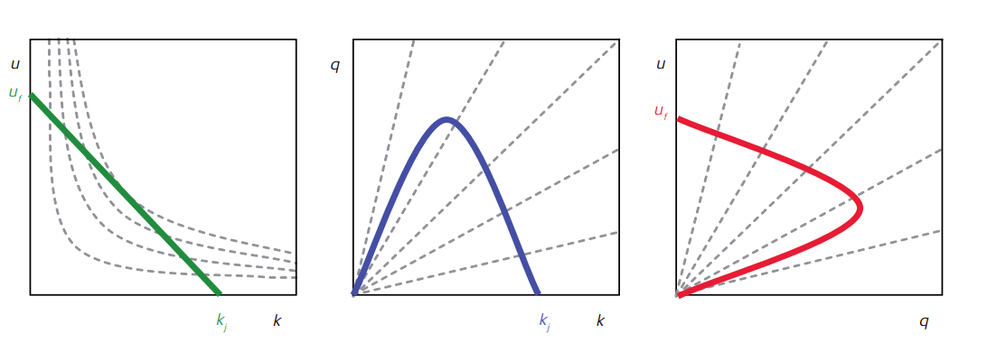
Figure 1: Fundamental diagrams of traffic flow, see [Notley2009].
In this section we will consider the most important relationships. Many more details, including derivations can be found in [books]. Before we start, units, the speed in metric systems is typically km/hr, and obviously miles/hr in imperial-based systems. Units: Speed is well well known and has the upper bound at the speed limit + some margin. Flow is often, but not exclusively, vehicles per hour, and usually ranges from 0-8000, density is veh / km.
The first and simplest relationship is the linear speed-density one formulated in 1935 by Greenshields [Greenshields1935]. k is the density, and u the average speed. The kj is the jam density and the uf is the free flow speed. The relationship is:
u = uf (1- k · kj) (4)
From a driver perspective the equation implies that drivers choose their speed according to the traffic density around them. The maximum speed is at 0 density, and conversely the minimum at maximum density.
The second is flow-density. A clearly non-linear relationship for varying speeds. At x=0, there are no vehicles, hence no density, k=0, therefore no flow (recall q=k·u). At maximum density (back to back) there is no flow as u=0, again no flow.
At fixed speeds this produces the straight dashed lines. In the case of the one with highest gradient is sometimes called the free-flow case, essentially the density or congestion does not interfere with the desired speed of the driver. From empirical data up the optimal density this essentially holds. One can see that there is a maximum density k* at which the density maximises the flow. In road planning cases this is where the road ‘should’ operate, less implies potentially underused capacity and higher densities implies congestion.
The third relationship couples speed and density. Essentially, the relationship between flow and average speed, where the upper portion of the curve can be interpreted as a free flow region, and the lower part represents congestion. This relationship does not constitute a mathematical function, as a single x values yields multiple y values.
Density, speeds and colourmaps

A fourth relation is speed-density, where at particular densities the speed slows and then collapses. In traffic flow terms, it is known as flow breakdown. Plotting the x axis on a log scale shows this effect more clearly as the speed density is more like a 2-piece linear relation and a ‘knee’ or inflection point where the speed does breakdown.
Averaging and windowing
The basic time resolution in traffic theory is the minute. Data collation, not collection, is often at this minute resolution. From each minute to hours, days to weeks some form of averaging or windowing is needed. Different time scales serve different purposes. Minute level-collations are processed hourly for rush-hour analysis. Daily aggregates are needed for weekday/weekend analysis etc.
Averaging traffic flow quantities is needed. The time-mean speed is measured at a MCS reference point on the roadway over a period of time. Average speed measurements obtained from this method are not accurate because instantaneous speeds averaged over several vehicles do not account for the difference in travel time for the vehicles that are traveling at different speeds over the same distance. The space-mean speed is measured over the whole roadway segment. Some form of monitoring tracks the speed of individual vehicles, and then the average speed is calculated. It is considered more accurate than the time mean speed. The time mean speed is never less than space mean speed:
Windowing is important as the intervals range from 1 to 1440 minutes per day. The length of a window can have significant effects on the outcomes, whether averages or visualisations. Since INRIX quantities are over a segment and MCS is a point, one or both of these might need to be averaged (over time).
Travel time
The average speed (u) is defined as the total distance divided by the total time, so
u =Travel distance (td) / Travel time (tt)
The average travel time (tt) over a distance l can be found as the average of the time a vehicle travels over a distance l:
mean(tt) = mean(1/v ) = l * mean(1v)
In this equation, tt indicates the travel time. This can be measured for all vehicles passing a road stretch, for instance at a local detector. Note that the mean travel time is not equal to the distance divided by the mean speed:
l * mean(1/v) l *1/mean(v)
In fact, it can be proven that in case speeds of vehicles are not the same, the average travel time is underestimated if the mean speed is used.
l * mean(1/v) <= l *1/mean(v)
The harmonically averaged speed, 1 divided by the average of 1 divided by the speed, provides a good basis for the travel time estimation. The pace Pi, is
Pi=1vi
The harmonically averaged speed is:
mean(v)harmonically = 1mean(Pi)= 1/1vi
The same quantity is required to find the space mean speed. We will see the travel time as an important quantity for the INRIX data. This is because INRIX speed is a segment (over a distance) measurement.
Simple traffic models
Using the logarithmic relationship between density and speed, Greenberg proposed [Greenberg1959]
u = uc * ln(kj * k)
Where,
k=density
kj=jam density
u= speed
uc=critical speed
An earlier linear version, 1935, is sometimes used
u = ur(1 – k * kj)
Where, ur = critical speed
Duncan’s model
u = qr(1/k – 1/kj)
Flow as density = outflow – inflow
uw = qdn -qupkdn – kup
Traffic data collection
Road traffic measurements are performed by many different stakeholders: government agencies, municipalities, researchers and commercial companies. The measurements are done for many different reasons, on different time scales, and with different techniques. See for instance Allström et al [Allström2017] and Sharma et al [Sharma2017] for an overview of traffic sensors and data collection techniques.
Government agencies and municipalities often measure road traffic for planning of future roads, for operation and maintenance, and for analysis of accident risks and environmental impact. The timescale of interest is often days, months or years. But sometimes measurements are also collected and used in real-time for traffic control and incident detection. The measurement techniques often include inductive loops, radars or pneumatic tubes. The Swedish Transport Administration, “Vägverket”, measures road traffic on the government owned roads in Sweden. They measure for instance traffic volume, “trafik arbete”, expressed in vehicle kilometers, to understand the usage of the road network. In order to monitor traffic trends in the country over time, the Swedish Transport Administration continuously measures traffic on about eighty road sections. These roads are selected to represent the entire state road network in Sweden. Complementary sampling is also done on many other stretches of road.
Several commercial companies, including Google, Waze, Here, TomTom, INRIX and many others, today collect and provide traffic information to drivers (and in some cases also to automotive companies, cities and road authorities). As an example, Google Traffic relies on crowdsourcing from drivers to collect traffic information. Google collects GPS information from phones and calculates the speed of the users on the road. In 2007, Google started to offer live traffic information on top of Google maps. A colour code (green, orange, red) is used to highlight the speed of traffic on a road: green means no traffic delays and the darker the red the slower the traffic on the road. Waze also relies on crowdsourcing from drivers to provide a real-time traffic service. They collect map and traffic information, and also allow users to report incidents on the road via a phone app [WAZE]. Google bought Waze in 2013. INRIX provides traffic information to road authorities, cities, automotive industries and individuals. They collect traffic data from many sources including road sensors, connected cars and mobile devices [INRIX]. The INRIX data is described in more detail in Section 2.1.1 of this report. Here Technologies is another example of a company that provides map, traffic and location services to both companies and individuals [HERE]. Also telecom companies collect data about traffic and mobility and provide services based on the data. In Sweden an example of this is Telia Crowd Insights [Telia].
New technology opens up for new innovative ways of measuring traffic. This includes video and cameras, Bluetooth and wifi measurements [Forsman2018], the use of drones, and connected cars talking to each other and the road infrastructure. Techniques that use Bluetooth or wifi are common for Automatic Vehicle Identification (AVI). The Bluetooth or wifi addresses of devices in cars are captured by roadside equipment. The same vehicle can in this way be identified at several locations; and this can be used to calculate travel time.
Alternative sensor data like vehicle probe data is much cheaper to collect, compared to traditional stationary sensors like radar and inductive loops. Also, with the new sensors a much larger part of the road network can be monitored. But there is an important difference in what type of data the different methods can provide. Vehicle probe data can provide speed and travel time but typically not traffic flow data. If flow data is needed as input to algorithms for traffic control or other calculations, then there is a need to estimate the flow from speed or travel time data. This estimation problem is the focus of the work in this report. Previous research on this estimation problem is surveyed by Seo et al. [Seo2017].
Traffic flow in practice
Traffic flow on a motorway is often very predictable from day to day. There is little traffic during night, and there are rush hours in the mornings and afternoons during weekdays. The pattern is a bit different during weekends and holidays with less traffic in the mornings. The average speed on the road follows a similar daily cycle. There are high speeds (around the speed limit) during night and during other free-flow periods, and low speeds when there is congestion during the rush hours. The figures below show how the traffic flow and average speed varies over one week on a motorway section in Stockholm (in October 2018).


The daily and weekly traffic pattern can of course vary between different motorways. Not all motorways have congestion during rush hours. Some roads have lower speeds during night because there is a large share of slower trucks and heavy traffic on the road at that time, etc. The amount of traffic and the average speed may also depend on the weather and the road conditions. For instance, with lower speeds during winter when there is snow and slippery roads. The traffic pattern on a motorway (with daily and weekly cycles) is in general very predictable. But it can also change both temporarily and over a long period of time. It is therefore important to continuously monitor the traffic. The traffic can change on an hourly basis due to accidents or sport events or weather conditions. It can change for weeks and months due to road works (or as a more unusual example: due to a pandemic). There are also many long-term trends and political decisions that might influence the traffic flow on a road. Just a few examples: more people are moving into the cities which means more traffic. New residential areas are built but also new alternative roads (that in some cases move away traffic from the cities). There is a trend to go by bike or use public transport instead of going by car, for environmental reasons. And there are political decisions like road tolls that influence the traffic pattern in a city.
In Section 1 we learned about fundamental diagrams and the theoretical relation between speed and flow on a road. In practice the relation between speed and flow can vary between different roads. The figure below shows a scatter plot of speed versus flow for the Stockholm motorway section (and the same week) as we looked at above.
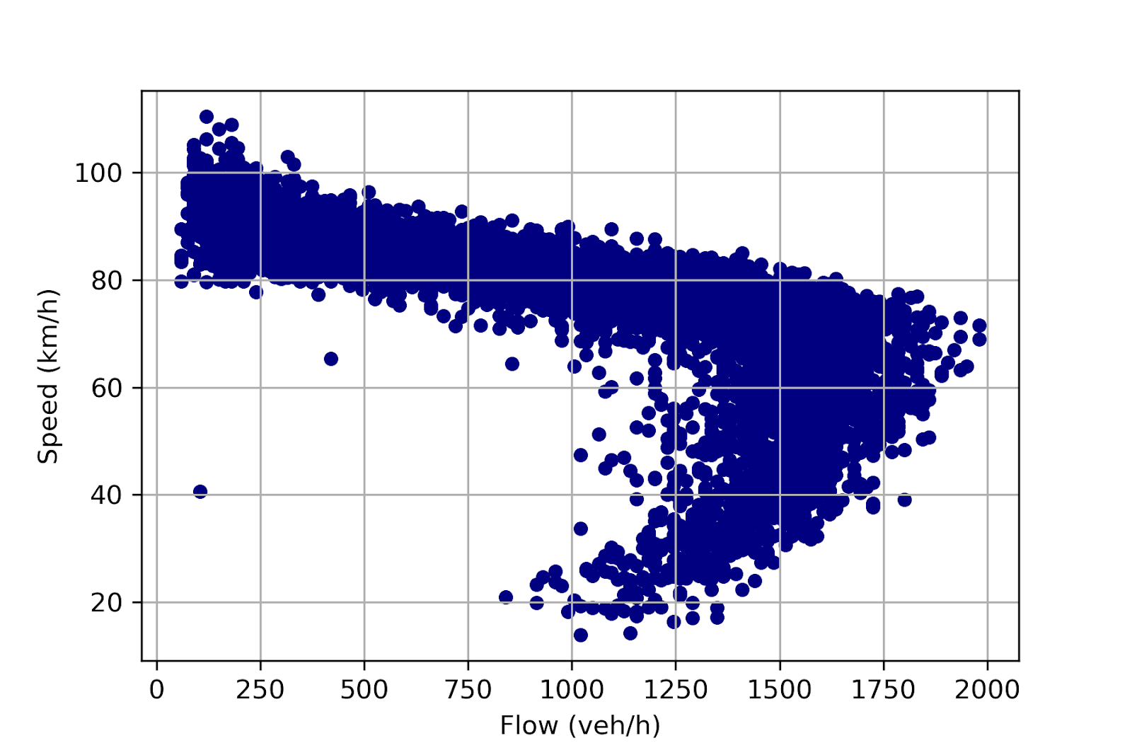
In the scatterplot below we can also see how the relation between speed and flow depends on the time of day. Here the color represents the hour of the day (0-23).

Blandin et al. studied the empirical relation between point speed and point flow for 112 stationary traffic radars in the San Francisco Bay Area, California [Blandin2012]. Their empirical measurements show that in reality the speed-flow relation can look very different at different roads (flat, increasing linearly, decreasing linearly, non-linear).

Data-driven examples
Maps, mapping and geographic information systems (GIS)
GIS are an essential part of any digitised traffic system. They capture, store, check, and display data related to positions on the Earth’s surface. GIS typically show streets, roads, buildings on maps. Whether for placement of sensors, attaining positions, plotting gathered data or visualising predictions we need mapping for the front end and the GIS system itself for the backend, processing and more. Commercial mapping tools that are well known include Google, WAZE, INRIX andHERE maps. For travel planners, some use an open file system, GTFS from Google originally, for timetabling. OpenStreetMaps is an open mapping system, and besides the core maintenance, relies heavily on user contributions. REST APIs are also open and can be built into applications such as [HereMaps].
Data sources with examples
INRIX
“Founded in 2005, INRIX pioneered the practice of managing traffic by analyzing data not just from road sensors, but also from vehicles. This breakthrough approach enabled INRIX to become one of the leading providers of data and insight into how people move around the world.” https://inrix.com/about/ (viewed 5 June 2020).
INRIX combines data from many sources to provide traffic information. A major part of the data comes from a crowdsourced model where INRIX continuously collects speed and location from probe vehicles, combines the data into an updated view of the current traffic situation on the road, and sends it back to the vehicles. In a press release back in May 2010 INRIX said they had a network of two million GPS-enabled vehicles: “Providing a foundation of continuous real-time speed and location reports to INRIX every minute for an average of 7 hours per day, per vehicle, commercial fleets – such as taxi cabs, service delivery vans and long haul trucks – represent the majority of INRIX’s network. INRIX intelligently combines these reports with data from consumer vehicles and GPS-enabled smartphones to deliver a service that updates traffic information to drivers every minute, ensuring they have the most accurate view of traffic conditions wherever they go.” Since that press release in 2010 the number of data sources that INRIX uses has grown significantly. In another press release In February 2014 INRIX highlighted its partnership with mobile operators to provide population flow analysis. They say: “We have spent a decade refining and patenting algorithms that are capable of integrating and interpreting mobile data with INRIX’s crowdsourced network of GPS, road sensor and connected car data sets”. And on the website today (June 2020) the company says they are “leveraging 500 Terabytes of INRIX data from 300 million different sources covering over 5 million miles of road.”
| Name | segmentid | timestamp | segment-type | speed | average | reference | traveltime(minutes) | score | cvalue | speedbucket |
| Range | ||||||||||
| 225285973 | 2018-10-01 00:00:14 | XDS | 93 | 60 | 60 | 0.332 | 30 | 49 | 3 | |
| 225285973 | 2018-10-01 00:01:12 | XDS | 93 | 60 | 60 | 0.332 | 30 | 50 | 3 | |
| 225285973 | 2018-10-01 00:02:10 | XDS | 93 | 60 | 60 | 0.332 | 30 | 50 | 3 |
Table 1: Example of INRIX speed data
Description of fields:
- segmentid: Unique identifier for the segment. The value would be the TMC code or the INRIX XD Segment ID.
- timestamp: measurement timestamp (GMT)
- segmenttype: Indicates type of segment. Possible values are TMC and XDS. XDS refers to a segment type of INRIX XD segment.
- speed: Current speed on the segment
- average: The typical speed on the segment for the given day and time
- reference: The free flow speed on the segment for the given day and time
- traveltimeminutes: Travel time along the segment at current speed in minutes
- Score: measure of confidence (see below)
- Cvalue: measure of confidence (see below)
- speedbucket: Level of congestion
INRIX provides two measures of confidence in the data: a Confidence Score and a Confidence Value (Score and Cvalue in the table above). Kim and Coifman [Kim2014] gives the following explanation:
“INRIX reports two measures of confidence in a given reported speed. The first measure INRIX calls the Confidence Score, in which INRIX assigns one of three possible outcomes: 30: High confidence, indicating that the report is based on real-time data for that specific segment. 20: Medium confidence, indicating that the report is based on real-time data across multiple segments and/or based on a combination of expected and real-time data. 10: Low confidence, indicating that the report is based primarily on historic data. […] INRIX reports a second measure of confidence, which they call the Confidence Value. Reportedly, the Confidence Value is based on a comparison against historical trends, though the details of this evaluation are proprietary. The Confidence Value only applies when the Confidence Score is 30.”
Several studies have evaluated INRIX probe data and compared it to concurrent roadside stationary measurements such as loop detectors and radar sensors. The API to the INRIX traffic data is public but how the data is collected is proprietary, and so is also the algorithms used for calculating speed and quality metrics. Many research studies on INRIX-data therefore include some reverse engineering, trying to figure out how the different metrics are implemented.
Kim and Coifman evaluate INRIX speed data by comparing it against concurrent loop detector data [Kim2014]. They study two months of data from an urban Interstate freeway in Columbus, Ohio, USA. The paper shows that, at a timescale of five minutes, both plots of the INRIX data and corresponding plots derived from loop detector data show similar patterns of congestion. The authors conclude that INRIX data works well for monitoring traffic but they point out three issues with the data: First, INRIX exhibited a latency of about 6 min compared to the loop detector data. Second, INRIX reports speed every minute, but most of the time the reported speed is identical to the previous sample, which indicates that the speed is calculated over a longer time period. Third, the INRIX confidence measures do not appear to reflect the latency or repeated measures. Kim and Coifman note that since the INRIX process is proprietary, there is no way to know if the INRIX data stream includes measurements from the same sensors that the study uses for evaluation. Comparisons between INRIX data and loop detector data should be viewed in this context. In this report we most often assume that the INRIX speed values are based on probe data and calculated from the GPS speed in vehicles.
Sharma et. al. studied INRIX probe data used for traffic operations and safety management in the state of Nebraska, USA [Sharma2017]. They evaluated INRIX-data against PVR (per vehicle record) sensor data. There are two main conclusions in their report: First, there is almost always a speed bias between data streaming from probes, the INRIX data and traditional infrastructure-mounted sensors. The average speed bias for real-time data reported in this work was 6.06 mph which is 9.75 km/h. The second conclusion is that lack of confidence score of 30 real-time INRIX probe data is a critical issue that needs to be considered when doing traffic analysis.
Ahsani et al explores the coverage of INRIX real-time data in the state of Iowa, USA, and demonstrates the growth in real-time data over a 4-year timespan [Ahsani2018]. A comparison is made with Wavetronix smart sensors to evaluate INRIX’s speed data quality. The paper investigates speed bias: the difference in speed values between the INRIX data and the Wavetronic sensors. Some differences are inevitable due to the differences in data collection methods. INRIX and other probe technologies calculate space mean speed; that is the average speed of vehicles over a length of road. Wavetronix, and other stationary road sensors, instead calculate time mean speed; which is the arithmetic mean of vehicles’ speed passing a given point. The paper shows that the speed bias may also depend on speed, segment length and time of day. Ahsani et al also study how accurate and reliable INRIX is when it comes to detecting congestion (both recurring and non-recurring).
The Motorway Control System (MCS)
The traffic flow in Stockholm is monitored with a Motorway Control System (MCS). A large number of stationary MCS-portals (gantrys) have been installed on the E4 and other roads. The MCS-portals are equipped with radar detectors and they monitor the flow and speed of traffic in each lane of the road. The data gives the regional traffic control centre information about the current traffic flow and speeds. The data is also input to a control system that sets variable speed limit signs. The radar measurements are point measurements and give time-mean-speed. This is in contrast to probe measurements such as INRIX calculate speed over a distance and provide space-mean speed, see Section 1.3.
The Stockholm Motorway Control System, including the subsystems for Variable Speed Limits (VSL) and Automatic Incident Detection (AID), is described in [Nissan2010], Section 3.2, pp 48-62].
Example of MCS data:
| fk_id | date | Speed (m/s) | speed_std_dev | Flow (cars/h) | used_lanes |
| 1159 | 2018-10-01 00:00:00 | 26.6028 | 7.1894 | 165 | {1,1,1,1} |
| 1159 | 2018-10-01 00:01:00 | 26.06 | 4.10961 | 160 | {1,1,1,NULL} |
| 1159 | 2018-10-01 00:02:00 | 25.0705 | 9.05539 | 105 | {1,1,1,1} |
Temporal factors
In addition to factors such as speed and density, which affect flow rate based on traffic theory, studies also found that the relations between flow and speed/density are in fact not static but changes with time, ie, dynamic. Dervisoglu et al. found that the maximum flow rate of a road segment not only changes on different days, but also changes before and after the congestion occurs under the same critical density, which means the flow-density relation in a road segment [Dervisoglu2009]. Duan also found that the flow rate patterns in weekends are different from patterns in weekdays, and using the data with different temporal factors when training could improve the performance of flow data imputation [Duan2016]. In this work, we also observed that the relation between flow and speed is different between daytime and night, i.e., a flow drop is observed under the same speed between daytime and night. Therefore, including the temporal factor of daytime/night into our feature vector should help the regression models to estimate the flow rate more precisely.
Spatial factors
Previous studies showed that traffic state parameters such as speed and flow rate of road links have spatial correlation with each other, which means that there are dependencies between different road links in the same road network and their traffic states are influenced by their neighbours [Ermagu2017]. Based on these observations, various studies have utilised the spatial dependency between road links in the problems of traffic state estimation and prediction. For example, Chen estimated/imputed the missing flow rate data of the detector by using data collected from neighbour detectors (in the same timestamp) based on the linear relations of flow rate between the center and neighbour detectors [Chen2003]. Among spatial relations between road links, strong positive correlations were observed between the links and their upstream/downstream links [Ermagu2017]. For example, Duan et al. found that the accuracy of their flow estimation model could be improved by including the data from upstream and downstream road segments instead of only using the data from a single road segment as the input feature [Duan2016]. Moreover, the spatial correlation between road links, especially the positive correlations between target links and their immediate upstream/downstream links, are widely used to solve the traffic prediction and estimation problems [Zhang2019, Ermagu =2017].
In this work, we also observed a high correlation of INRIX data between south and north road segments at the same time step (correlation > 0.95). Therefore, we consider the spatial factor by including INRIX data from the adjacent road segment into our model. By doing so we expect to improve the accuracy of estimation since the data from the upstream/downstream segments may provide extra information about traffic states based on the spatial correlation.
Data-driven models of traffic flow
Parametric models
Existing approaches for estimating traffic state can broadly be divided into two kinds, parametric models such as time series models and state-space models. Parametric models assume some (finite) set of parameters θ. Given these parameters, future predictions x are independent of the observed data, D:
P( x | θ, D) = P(x | D)
Parameters include the location, mu in the Normal N(𝜇, 𝝈2) distribution, or a dispersion parameter the 𝝈 in N(𝜇, 𝝈2) normal again. Some distributions have a shape parameter, such as the Gamma or Beta distributions.
Non-parametric models
Non-parametric models of traffic flow assume that the data distribution cannot be defined by a finite set of parameters. Sometimes one can think of an infinite dimensional θ, the amount of information that θ can capture about the data D can grow as the amount of data grows, which can be more flexible. Essentially this report is about non-parametric models, as we use data-driven, and not 2-3 parameterised functions to estimate traffic flow.
Nikovski compared non-parametric KNNs, regression trees, locally-weighted regression and neural networks to predict the short-term travel times in [Nikovski2004]. Duan used an autoencoder to impute/estimate the missing flow data from traffic sensors, and compared its performance with other non-parametric models, e.g., linear regression and back-propagation neural networks [Duan2016]. Other non-parametric models include k-nearest neighbours, neural networks, deep learning and so on [Lint2012, LV2015, Ma2015, Polson2017, Zhao2017, Li2017].
Linear regression
Linear regression belongs to the non-parametric methods for solving traffic prediction/estimation problems as both the model structure, the number of independent variables or degree of polynomial, and values of the parameters, the intercept and coefficient of each dependent variable, are determined from the historical data. Linear regression uses historical data to fit a function that characterizes how each covariate, known as the independent variables, influences the outcome variable known as the dependent variable. This linear function is then used to estimate/predict the flow, speed, density, based on unseen data.
Many studies use linear regression as a baseline model to compare with some more sophisticated models, such as neural networks, for traffic flow prediction [Lint2012]. Kwon et al. use a linear regression model to predict future travel time based on data from loop sensors such as the flow and occupancy, and probe sensors from the departure times and week days [Kwon2000]. Nikovski et al. also used a simple linear regression model with 1 to 3 most recent travel times as input variables to predict the travel time in a short-term future [Nikovski2004].
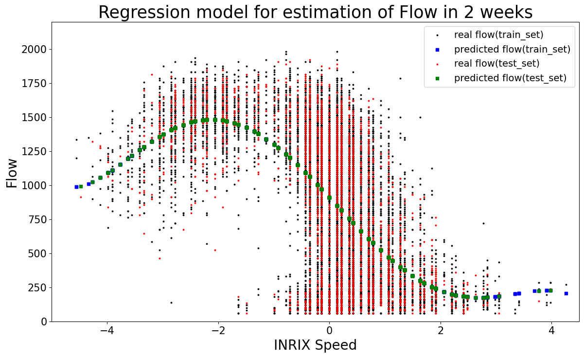
Figure 3: Linear regression model for estimating macroscopic flow from INRIX speed.
Some studies also adopted linear regression models to estimate traffic states based on partially observed spatial data [Seo2017]. For example, Chen et al. used a linear regression model to estimate the missing data for loop sensors based on traffic data from neighbouring sensors around the sensor with missing data [Chen2007].
Although linear regression models for traffic prediction are sometimes outperformed by nonlinear models in traffic flow prediction due to the nonlinear nature of traffic flow, its computational efficiency and low memory usage still give it an competitive edge while short execution time is a critical requirement. Moreover, linear regression models sometimes show comparable accuracy in predicting traffic flow as other nonlinear models [Nikovski2004]. In this project, linear regression models mainly serve as baseline models for performance comparison with other models. For example, we use linear regression as one of ML models to describe the relation between INRIX data and macroscopic traffic flow in MCS data, which is shown in Fig. 3.
Hybrid models
Parametric and non-parametric traffic models can also be combined. Parametric and nonparametric traffic state prediction techniques have previously been developed with different advantages and shortcomings. While nonparametric prediction has shown good results for predicting the traffic state during recurrent traffic conditions, parametric traffic state prediction can be used during nonrecurring traffic conditions, such as incidents and events.” In this paper, parametric and nonparametric traffic state prediction techniques are […] combined through assimilation in an ensemble Kalman filter. For nonparametric prediction, a neural network method is adopted; the parametric prediction is carried out with a cell transmission model with velocity as state.” [Allström2106].
Estimating traffic flow from probe data
Traditionally, traffic has been measured with expensive stationary road sensors that provide information about flow, speed and occupancy. These sensors are sometimes referred to as eulerian sensors. Traditional traffic models have been developed based on this data, and therefore often need flow or density as input. But today it is common to collect data from probe vehicles (i.e. gps-equipped cars and smartphones). Probe vehicle data is sometimes also called mobile data, floating car data (FCD) or Lagrangian data. That data is continuously gathered from the vehicles while driving. The data gives information about speed and traveltime, but it does not typically give any flow information. Given this new type of data, researchers are trying to: (a) adapt or create new traffic models that incorporate probe data; and (b) find methods to derive traffic flow from vehicle probes that measure speed and travel time [Seo2017].
Using fundamental diagrams to estimate flow from probe speed data
One common approach to estimate the traffic flow from probe data is to use a fundamental diagram (see Section 1.2.1) that provides the relationship between speed and flow for a specific road. Given speed data the flow can, at least in principle, be calculated. But mapping from speed to flow using a fundamental diagram can be challenging, especially in the free-flow phase [Herrera2010, Blandin2012, Anuar2016, Seo2017].
Blandin et al studied the empirical relation between point speed and point flow for stationary traffic radars in the San Francisco Bay Area, California [Blandin2012] . They studied stationary measurements but the goal, in the end, was to assess the feasibility of inferring traffic flow from probe speed. The authors emphasise that in classical traffic flow theory, using the fundamental relationships, velocity is constant (at the free-flow speed) in the uncongested phase. If the spacing between vehicles is large enough, the drivers will not be constrained by the surrounding vehicles, and so they can travel at free-flow speed. This means that in the uncongested phase, conversion from speed to flow is theoretically impossible as speed is theoretically constant at the free-flow speed. However, Blandin et al show with empirical measurements from radar stations that in reality the speed-flow relation can look very different at different roads (flat, increasing linearly, decreasing linearly, non-linear). Blandin et al use linear regression to estimate flow from speed, calibrating the model using historical stationary data. They also investigate regression of flow over speed variance. The paper concludes that the proposed methods give reasonably accurate flow estimates, and that the conventional speed-flow method gives significantly more accurate results than the speed variance-flow method.
Using probe data raises a number of additional issues to consider: A basic question with the FD approach is how a well-calibrated fundamental diagram is created. If the objective with probe measurements is to replace expensive stationary measurements, then it doesn’t work to use loop-detector data to provide a good FD. A fundamental diagram from another road in the same category might then be used, if it can be assumed to be similar enough. There are also efforts to derive the FD without stationary measurements. For instance, Seo et al [Seo2019] present a framework for estimating the fundamental diagram without stationary detectors. Instead they use only probe data and information about the jam density.
The aggregation interval of the speed data is often also an important issue. It is also important to consider how representative the speed of the probe vehicles are, compared to all traffic. How large share of the vehicles on the road provides speed data (the penetration rate)? Do we mostly get values from a fleet of slow trucks and/or fast driving taxis? Another issue to consider is that probe techniques provide space-mean speed while stationary sensors would give time-mean speed. The characteristics of a specific road segment can also influence the speed and flow estimates (ramps, variable speed limits etc.) compared to measurements at a fixed point.
Herrera and Bayen [Herrera2010] propose two methods to incorporate speed measurements from vehicles into flow models for traffic state estimation purposes: a Kalman filtering technique and a Newtonian relaxation method. The latter technique modifies the Lighthill–Whitham–Richards partial differential equation to include a correction term which reduces the discrepancy between the probe measurements and the estimated state. Converting speed measurements into density using a fundamental diagram introduces some errors. However, the paper concludes that despite this error the proposed methods produce accurate estimates.
[Neumann2013a] derive traffic volumes from probe vehicle data by applying the speed-flow relationship of the fundamental diagram (using the van Aerde model) on hourly averaged data. Evaluation is done with data from 600 local detectors and a taxi fleet with 4300 vehicles in Berlin, Germany. In [Neumann2013b] the authors say that the approach in [Neumann2013a] is “more or less applicable, in principle”, but the deterministic modelling of the speed-flow relation does not capture the variations in speeds given the same traffic flow. [Neumann2013b] proposes a more detailed representation of the fundamental diagram (speed and flow) based on Bayesian networks which also takes into account the dynamic transitions between traffic states over time.
K. A. Anuar estimates traffic volume from probe vehicle data specifically for freeways in the Ph.D. thesis [Anuar2016]. Fundamental diagrams is one of three methods explored in the thesis (the other two approaches being: shockwaves and information about the space headway between lead and follower vehicles). The thesis studies four different fundamental diagrams (Greenshields, Underwood, Northwestern, Van Aerde) and data aggregated in 5, 10 and 15 minutes intervals. The results using fundamental diagrams are also presented in the paper [Anuar2015]. The probe vehicle data used in this study comes from the Mobile Century project in San Francisco (2008) where GPS data (timestamp and position) was collected from vehicles with recruited drivers. The estimated traffic flows are compared to measured traffic flows from loop detectors. In this case study the Van Aerde-model provides the best results. It gives reasonable estimates of traffic flow rates with good estimates during periods of high flow rates, and with slight underestimation during medium flow rates. Aggregating the data into 15-minutes intervals smoothens the data and gives lower estimation errors. Traffic flow rates are more accurately estimated during congested traffic conditions compared to free-flow conditions in this study.
FD-free flow estimation using extended mobile data or limited stationary data
There are also methods that estimate flow from mobile measurements without using a fundamental diagram. These methods often either (a) combine mobile measurements with vehicle counts and other limited stationary data [Seo2017, Coifman2003, Astarita2006, Qiu2010, Bekiaris-Liberis2016, Nanthawichit2003, Sekula2017] or (b) make use of more advanced mobile data (than just speed and travel time), for instance spacing information [Seo2015a, Seo2015b, Anuar2016] .
Related Work
Mobile Century and Mobile Millennium [MobileMillenium, Bayen2011] were influential projects at University of California, Berkeley, in 2008-2011. Mobile Millennium was a research project that included a pilot traffic-monitoring system that used the GPS in cellular phones to gather traffic information, process it, and distribute it back to the phones in real time. The objective of the project was to demonstrate the potential of GPS in cell phones to alter the way traffic data is collected. The Mobile Millennium Stockholm-project [Allström2011] studied methods for data fusion. The project adapted and extended the knowledge gained from the Mobile Millennium project at Berkeley in order to estimate travel times in Stockholm. Examples of how methods developed in the Mobile Millennium Stockholm-project are used to estimate traffic state can for instance be found in [Grumert2019].
Kim and Coifman evaluate INRIX speed data by comparing it against concurrent loop detector data [Kim2014]. It is one of two papers looking at floating and loop data. They study two months of data from an urban Interstate freeway in Columbus, Ohio, USA. The paper shows that, at a timescale of five minutes, both plots of the INRIX data and corresponding plots derived from loop detector data show similar patterns of congestion. The authors conclude that INRIX data works well for monitoring traffic but they point out three issues with the data: First, INRIX exhibited a latency of about 6 min compared to the loop detector data. Second, INRIX reports speed every minute, but most of the time the reported speed is identical to the previous sample, which indicates that the speed is calculated over a longer time period. Third, the INRIX confidence measures do not appear to reflect the latency or repeated measures. They shift the floating vehicle measurements to maximise the correlation coefficient of the speeds. Given the travel time across the segment, and the segment length it is not totally clear if shifting the speeds to identical positions in time is not clear. 3) Similar to us: In that they consider floating and loop detector traffic flow measurements. 4) Different from us: TBD. 5) Findings compared to us.
Sharma et al. summarise the experiences and lessons learned while using probe data for traffic operations and safety management in the state of Nebraska, USA [Sharma2017]. This work evaluates INRIX-data against PVR (per vehicle record) sensor data. The report gives an overview of related work and reviews the different performance measures used for INRIX data in the literature. The report also gives a review of different sensor technologies. There are two main conclusions in the report. First, there is almost always a speed bias between data streaming from probes (the INRIX data) and traditional infrastructure-mounted sensors. The average speed bias for real-time data reported in this work was 6.06 mph (9.75 km/h). The second conclusion is that lack of confidence score 30 (real-time) INRIX probe data is a critical issue that needs to be considered when doing traffic analysis.
The paper by Ahsani et al. explores the coverage of INRIX real-time data in the state of Iowa, USA, and demonstrates the growth in real-time data over a 4-year timespan [Ahsani2018] . A comparison is made with Wavetronix smart sensors to evaluate INRIX’s speed data quality. The paper investigates speed bias: the difference in speed values between the INRIX data and the Wavetronic sensors . Some differences are inevitable due to the differences in data collection methods. INRIX (and other probe technologies) calculate space mean speed; that is the average speed of vehicles over a length of road. Wavetronix, and other stationary road sensors, instead calculate time mean speed; which is the arithmetic mean of vehicles’ speed passing a given point. The paper shows that the speed bias may also depend on speed, segment length and time of day. Ahsani et al also study how accurate and reliable INRIX is when it comes to detecting congestion (both recurring and non-recurring).
The report by Grumert et al. evaluates different control algorithms that determine which speed limits that are going to be displayed on variable message signs on two motorway sections in Stockholm [Grumert2019]. In addition, the report studies how estimated traffic conditions can be used as a complement to fixed detectors installed along the road. The Mobile Millenium Stockholm (MMS) system, which consists of a macroscopic traffic flow model and Kalman filtering for prediction and estimation of traffic states, has been used to estimate traffic states. The relation between speed and density (and also flow) is in this kind of model described with a fundamental diagram. The fundamental diagram used in this study has a linear shape during free flow and a hyperbolic shape during congestion. Calibration of three parameters is needed to adapt the model for each specific road segment.
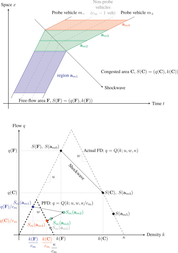
The Fundamental diagram (FD) contains useful information on traffic features, e.g., flow capacity and identification of free flow and congestion regimes, and therefore is widely used in traffic flow modeling and traffic state estimation [Seo2019]. This paper proposes a theory framework as well as a computational algorithm to estimate FD by using probe vehicle data (trajectory and speed), which is a more cost-effective way to collect traffic data. Algorithm firstly uses probe pairs in steady state, i.e., vehicles exhibit the same constant speed, to determine 2 FD parameters, i.e., free flow speed and backward wave speed. In order to determine the shape of the FD triangle, it needs at least 1 steady probe pair in free-flow regime and 2 steady probe pairs in congestion regime, together with the origin traffic state that is already known. Secondly, it needs the parameter jam density, which is provided by additional data sources such as satellite or roadside detector, to determine the scale ratio between real FD and probe FD estimated by probe pairs. Some parameter combinations need to be fine tuned to generate enough data pairs in steady states, such as speed threshold for filtering non-steady state data pairs. The approach is validated by real-world probe data and generates good results that align to the data from loop detectors.
1. The approach in this work estimates the traffic flow (FD) based on theoretical models with much more complex computation and more parameter-tuning needs to be tailored to the individual dataset.
2. It uses trajectory of probe vehicles as features and traffic jam density as label (from loop detector or satellite photo) to build the model; while we currently use speed and travel-time from probe vehicles as features and flow/density from loop detectors as label to train the estimation model. 1. Although we may not need to manipulate trajectory data like this work did, trajectory data (space-time pairs) might still be a good resource to provide additional features for estimation/prediction in regression or RNN models. 2. Some filtering methods could be adopted to clean the INRIX data, e.g., set the upper bound of the speed to filter the data points with unrealistic values.
References
[HERE] Traffic Analytics, Rich location intelligence for more effective traffic management https://www.here.com/products/traffic-solutions/road-traffic-analytics>, viewed 4 June 2020.
[Ahsani2018] V. Ahsani, M. Amin-Naseri, S. Knickerbocker and A. Sharma (2018): Quantitative analysis of probe data characteristics: Coverage, speed bias and congestion detection precision, Journal of Intelligent Transportation Systems, DOI: 10.1080/15472450.2018.1502667 (pdf).
[Allström2011] Allström, A., Archer, J., Bayen, A. M., Blandin, S., Butler, J., Gundlegård, D., Koutsopoulos, H., Lundgren, J., Rahmani, M. & Tossavainen, O. P. Mobile Millennium Stockholm. Proceedings of the 2nd International Conference on Models and Technologies for Intelligent Transportation Systems, June 2011 Leuven, Belgium.
[Allström2016 ] Andreas Allström, Joakim Ekström, David Gundlegård, Rasmus Ringdahl, Clas Rydergren, Alexandre M. Bayen, and Anthony D. Patire, Hybrid Approach for Short-Term Traffic State and Travel Time Prediction on Highways, Transportation Research Record: Journal of the Transportation Research Board, No. 2554, 2016, pp. 60–68. DOI: 10.3141/2554-07. https://bayen.berkeley.edu/sites/default/files/hybrid_approach.pdf
[Allström2107] Allström, A., Barcelo, J., Ekström, J., Grumert, E., Gundlegård, D., and Rydergren, C. (2017). “Traffic management for smart cities”. In: Designing, Developing, and Facilitating Smart Cities. Springer, pp. 211–240. ISBN: 9783319449227 (Print), 9783319449241 (eBook) http://liu.diva-portal.org/smash/get/diva2:975199/FULLTEXT01, viewed 25 June 2020.
[Astarita2006] Astarita, V., Bertini, R.L., d’Elia, S., Guido, G., 2006. Motorway traffic parameter estimation from mobile phone counts. European Journal of Operational Research 175 (3), 1435–1446. doi:10.1016/j.ejor.2005.02.020
[Anuar2015] Khairul Anuar, Filmon Habtemichael, and Mecit Cetin. 2015. Estimating Traffic Flow Rate on Freeways from Probe Vehicle Data and Fundamental Diagram. In Proceedings of the 2015 IEEE 18th International Conference on Intelligent Transportation Systems (ITSC ’15). DOI:https://doi.org/10.1109/ITSC.2015.468
[Anuar2016] Anuar, Khairul A.. “Methodologies for Estimating Traffic Flow on Freeways Using Probe Vehicle Trajectory Data” (2016). Doctor of Philosophy (PhD), dissertation, Civil/Environmental Engineering, Old Dominion University, DOI: 10.25777/g4ym-b938, https://digitalcommons.odu.edu/cee_etds/13
[Bayen2011] Bayen, A., Butler, J. & Patire, A. D. 2011. Mobile Millennium Final Report. California Center for Innovative Transportation Institute of Transportation Studies University of California, Berkeley.
[Bekiaris-Liberis2016] Bekiaris-Liberis, N., Roncoli, C., Papageorgiou, M., 2016. Highway traffic state estimation with mixed connected and conventional vehicles. IEEE Transactions on Intelligent Transportation Systems 17 (12), 3484–3497.
[Blandin2012] Blandin, S., Salam, A., Bayen, A.M., 2012. Individual speed variance in traffic flow: analysis of Bay Area radar measurements, in: Transportation Research Board 91st Annual Meeting.
[Chen2003] Chen, C., J.Kwon, J.Rice, A.Skabardonis, and P. Varaiya. Detecting errors and imputing missing data for single-loop surveillance systems. Transp. Res. Rec., 1855, 160–167.
[Chen2007] Chen, Chao, Kwon, Jaimi, Rice, John, Skabardonis, Alexander and Varaiya, Pravin. (2003). Detecting Errors and Imputing Missing Data for Single-Loop Surveillance Systems. Transportation Research Record. 1855. 10.3141/1855-20.
[Coifman2003] Coifman, B., 2003. Estimating density and lane inflow on a freeway segment. Transportation Research Part A: Policy and Practice 37 (8), 689–701. doi:10.1016/S0965-8564(03)00025-9.
[Dervisoglu2009] Dervisoglu, G., Gomes, G., Kwon, J., Horowitz, R., Varaiya, P., 2009. Automatic calibration of the fundamental diagram and empirical observations on capacity, in: Transportation Research Board 88th Annual Meeting.
[Duan2016] Duan, Y., Lv, Y., Liu, Y.L., Wang, F.Y., 2016. An efficient realization of deep learning for traffic data imputation. Transportation Research Part C: Emerging Technologies 72, 168–181.
[Elefteriadou2014], Lily Elefteriadou, Introduction to traffic flow. Springer, 2014
[Forsman2018] Åsa Forsman, Anna Vadeby, David Gundlegård, Rasmus Ringdahl. Utvärdering av hastighetsmätningar med blåtandssensorer: Jämförelse med data från MCS (Motorway Control System), VTI rapport 969, 2018.
[Grumert2019] Ellen Grumert, Viktor Bernhardsson, Joakim Ekström, David Gundlegård, Rasmus Ringdahl and Andreas Tapani. Variabla hastighetsgränser för Stockholms motorvägsnät: effekter av alternativa algoritmer och möjligheter till styrning genom estimerade trafiktillstånd. The Swedish National Road and Transport Research Institute (VTI), VTI rapport 1006, 2019. (pdf)
[HERE] Here Technologies, “HERE Traffic Analytics: Rich location intelligence for more effective traffic management”,
[HereMaps] Guide – Maps API for Javascript, link.
[INRIX] AI Traffic: The Next Evolution of Traffic Intelligence to Help You Conquer Congestion. link.
[Kim2014] Seoungbum Kim, Benjamin Coifman, Comparing INRIX speed data against concurrent loop detector stations over several months, Transportation Research Part C: Emerging Technologies, Volume 49, 2014, Pages 59-72, ISSN 0968-090X, link.
[Kwon2000] Kwon, Jaimie & Coifman, Benjamin & Bickel, Peter. (2001). Day-to-Day Travel Time Trends and Travel Time Prediction from Loop Detector Data. Transportation Research Record: Journal of the Transportation Research Board. 1717. 10.3141/1717-15.
[Lana2018] I. Lana, J. Del Ser, M. Velez and E. I. Vlahogianni, Road Traffic Forecasting: Recent Advances and New Challenges, in IEEE Intelligent Transportation Systems Magazine, vol. 10, no. 2, pp. 93-109, Summer 2018, doi: 10.1109/MITS.2018.2806634. <link>
[Li2017] Li et al, link, ICLR, 2018.
[Li2017] Y Li, R Yu, C Shahabi, Y Liu. Diffusion convolutional recurrent neural network: Data-driven traffic forecasting, 2017, link.
[Lint2012] Van Lint and van Hinsbergen. Short-term traffic and travel time prediction models, Artificial Intelligence and Advanced Computing Committee, Transportation Research Board (Ed.), Transportation Research Circular. National Academies Press. E-C168, pp. 22–41, 2012.
[LV2015] Y. Lv, Y. Duan, W. Kang, Z. Li and F. Wang, Traffic Flow Prediction With Big Data: A Deep Learning Approach, in IEEE Transactions on Intelligent Transportation Systems, vol. 16, no. 2, pp. 865-873, April 2015, doi: 10.1109/TITS.2014.2345663.
[Ma2015] X. Ma, Z. Tao, Y. Wang, H. Yu, Y. Wang. Long short-term memory neural network for traffic speed prediction using remote microwave sensor data, Transportation Research Part C: Emerging Technologies, Volume 54, May 2015, Pages 187-197, paper.
[Duan2016] Duan, Y., Lv, Y., Liu, Y., & Wang, F. (2016). An efficient realization of deep learning for traffic data imputation. Transportation Research Part C: Emerging Technologies, 72, 168-181, link.
[Lana2018] surveys recent advances and challenges for road traffic forecasting, including data-driven procedures.
[Ermagu2017] Ermagun, A., Chatterjee, S., & Levinson, D. (2017). Using temporal detrending to observe the spatial correlation of traffic. PloS one, 12(5), e0176853. https://doi.org/10.1371/journal.pone.0176853
[MobileMillenium] Mobile Millennium http://traffic.berkeley.edu
[Nanthawichit2003] Chumchoke Nanthawichit,Takashi Nakatsuji and Hironori Suzuki, Application of Probe Vehicle Data for Real-Time Traffic State Estimation and Short Term Travel Time Prediction on a Freeway, Proceeding of 82nd TRB Meeting, Washington D.C., 2003.
[Neumann2013a] T. Neumann, L. C. Touko Tcheumadjeu, P. L. Böhnke, E. Brockfeld, and X. Bei, Deriving Traffic Volumes from Probe Vehicle Data using a Fundamental Diagram Approach, in Proceedings 13th World Conference on Transport Research, Rio de Janeiro, Brazil, 2013.
[Neumann2013b] Neumann, T., Böhnke, P.L., Tcheumadjeu, T., Louis, C., 2013. Dynamic representation of the fundamental diagram via Bayesian networks for estimating traffic flows from probe vehicle data, in: 2013 IEEE 16th International Conference on Intelligent Transportation Systems, pp. 1870–1875, link.
[Nikovski2005] Nikovski, Daniel and Nishiuma, N. and Goto, Y. and Kumazawa, H. Univariate Short-Term Prediction of Road Travel Times, 2005, Pages 1074 – 1079. 10.1109/ITSC.2005.1520200.
[Nissan2010] Nissan, Albania, “Evaluation of Variable Speed Limits: Empirical Evidence and Simulation Analysis of Stockholm’s Motorway Control System”, Ph.D Thesis, KTH, School of Architecture and the Built Environment (ABE), Transport and Economics, Traffic and Logistics. 2010, link.
[Notley2009] S. O. Notley, N. Bourne, N.B. Taylor. Speed, Flow and density of motorway traffic. UK TRL Insight report INS003, link.
[Polson2017] N. Polson and V. Sokolov, Deep learning for short-term traffic flow prediction, 2017, link.
[Qiu2010] Qiu, T., Lu, X.Y., Chow, A., Shladover, S., 2010. Estimation of freeway traffic density with loop detector and probe vehicle data. Transportation Research Record: Journal of the Transportation Research Board (2178), 21–29.
[Sekula2017] Przemyslaw Sekula, Nikola Markovic, Zachary Vander Laan, Kaveh Farokhi Sadabadi, Estimating Historical Hourly Traffic Volumes via Machine Learning and Vehicle Probe Data: A Maryland Case Study, 2017, link.
[Seo2015a] Seo, T., Kusakabe, T., 2015. Probe vehicle-based traffic state estimation method with spacing information and conservation law. Transportation Research Part C: Emerging Technologies 59, 391–403, link.
[Seo2015b] Seo, T., Kusakabe, T., Asakura, Y., 2015. Traffic state estimation with the advanced probe vehicles using data assimilation, in: 2015 IEEE 18th International Conference on Intelligent Transportation Systems, pp. 824–830. doi:10.1109/ITSC.2015.139.
[Seo2017] T. Seo, AM. Bayen, T. Kusakabe, Y. Asakura., Traffic state estimation on highway: A comprehensive survey, Annual Reviews in Control, 2017, paper.
[Seo2019] Toru Seo, Yutaka Kawasaki, Takahiko Kusakabe, Yasuo Asakura, Fundamental diagram estimation by using trajectories of probe vehicles, Transportation Research Part B: Methodological, Volume 122, 2019, Pages 40-56, ISSN 0191-2615, link.
[Sharma2017] A. Sharma, V. Ahsani, and S. Rawat, Evaluation of Opportunities and Challenges of Using INRIX Data for Real-Time Performance Monitoring and Historical Trend Assessment, 2017, Reports and White Papers. 24, link.
[Telia] Telia Crowd Insights, “How it works”, link, 2020.
[vanLint2012] van Lint and van Hinsbergen, Short-term traffic and travel time prediction models, 2012. This paper reviews neural network and AI applications to short-term traffic forecasting
[Vlahogianni2014] EI. Vlahogianni, MG. Karlaftis, JC. Golias. Short-term traffic forecasting: Where we are and where we’re going. Transportation Research Part C: Emerging Technologies, 43:3–19, 2014, paper.
[WAZE] <https://www.waze.com>, viewed 4 June 2020.
[Zhao2017] Z. Zhao, W. Chen, X. Wu, PCY. Chen, J. Liu. LSTM network: a deep learning approach for short-term traffic forecast, IET Intelligent Transport Systems, 2017, Volume 11 Issue 2, pages 68-75, paper.
MOBILE MILLENNIUM STOCKHOLM
Andreas Allström, Jeffery Archer, Alexandre M.’Bayenc, Sebastien Blandinc, Joe Butlerd, David Gundlegård, Haris Koutsopoulose, Jan Lundgren, Mahmood Rahmanie, Olli Pekka Tossavainen.
https://bayen.berkeley.edu/sites/default/files/cmt11.pdf
Mobile Millennium: GPS Mobile Phones as Traffic Probes, California Networked Traveler – Safe Trip 21 Phase II, link.
https://www.springer.com/gp/book/9781461484349,
https://doi.org/10.1007/978-1-4614-8435-6
Surveys of the different approaches are available. Vlahogianni et al. reviews existing research and identifies technological and analytical challenges for the next generation of short term forecasting research [Vlahogianni2014].
Van Lint and van Hinsbergen reviews neural networks and AI applications to short-term traffic forecasting [Lint2012].
[Zhang 2019] T. Zhang, J. Jin, H. Yang, H. Guo and X. Ma, “Link speed prediction for signalized urban traffic network using a hybrid deep learning approach,” 2019 IEEE Intelligent Transportation Systems Conference (ITSC), Auckland, New Zealand, 2019, pp. 2195-2200, doi: 10.1109/ITSC.2019.8917509.